Meta Surface: An Introduction
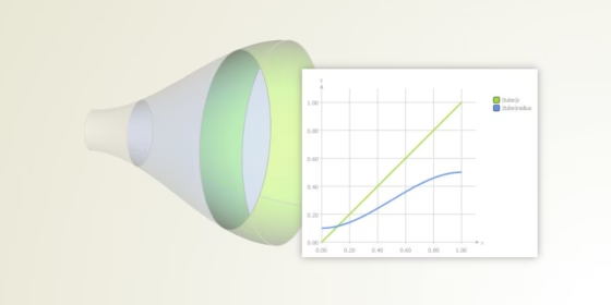
As a specialized CAD solution, CAESES provides a set of different surface types in order to create flexible parametric geometry models. The meta surface is a bit distinct, when you compare it to common surface types in other CAD systems. Basically, a meta surface is a parametric sweep surface with more user controls and hence a higher flexibility, especially in the context of efficient shape optimization with simulation tools. It allows you to massively reduce the total number of parameters, while always generating smooth and feasible surface shapes. In particular, meta surfaces are ideal for complex free-form surfaces such as ducts, wings, exhaust ports, volutes, blades, ship hulls etc., to foster innovation with more customized and ready-to-automate CAD models. This blog post introduces the concept of meta surfaces as a generalized technique for a broad variety of applications.
An Example
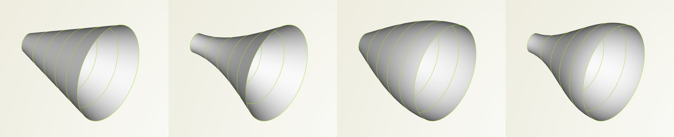
Let’s keep it simple and assume we want to design a variable tube geometry for which we would want to find an optimal shape, e.g. with regards to some flow characteristics. The following picture shows 4 different tubes:
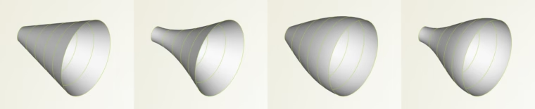
Different tube geometries where the radii values are varied
You can create such a tube in various ways: For instance, we could create a surface of revolution using a parametric contour. However, we want to extend this geometry later to be asymmetric, or even to sweep the tube along a 3D path. Hence, a surface of revolution is no option.
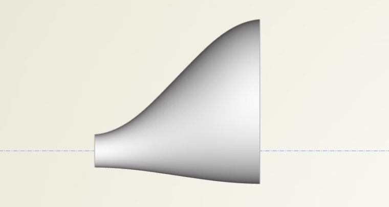
Be able to have a asymmetric tube or more complex shape later
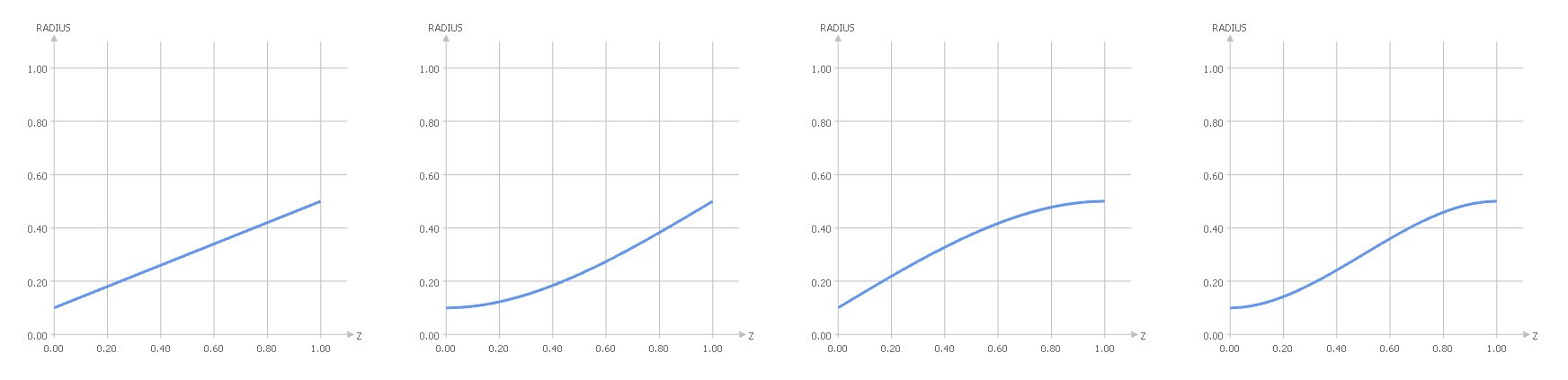
Another more generalized procedure is to create a set of 2D circles in the XY-plane, using different radii values at different z‑locations. These circles can then be interpolated by a surface using a NURBS skinning process. If we consider 6 circles for each tube as shown in the first picture, we can plot and interpolate the radii values to receive a distribution:
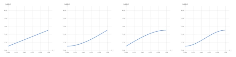
Corresponding radii distributions for the 4 different tube shapes
However, such a section-based surface creation process is typically tedious because there is a lot of manual cross-section creation and individual modeling required. On top of that, the modeling process can potentially create infeasible shapes, e.g. constraints need to be fulfilled and surface oscillations come up due to the interpolation. Last but not least, the entire workflow is not generalized and cannot be used for similar design tasks.
Meta Surfaces
Meta surfaces simplify the cross-section approach and introduces a fully generalized approach to such a standard task.
Meta Surfaces are parametric sweep surfaces, where the surface generation process is efficiently controlled by a set of function graphs.
The overall goal of meta surfaces is to give you the quick possibility to use function graphs for creating geometry variations. The graphs can be connected to design exploration and optimization strategies, so that the geometry generation process is automated and robust. This finally creates an efficient automated setup and makes sure that you create only nice, feasible shapes. Let’s take a closer look at how meta surfaces are set up in CAESES.
Step 1: Curve Definition
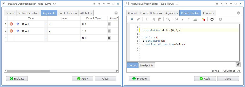
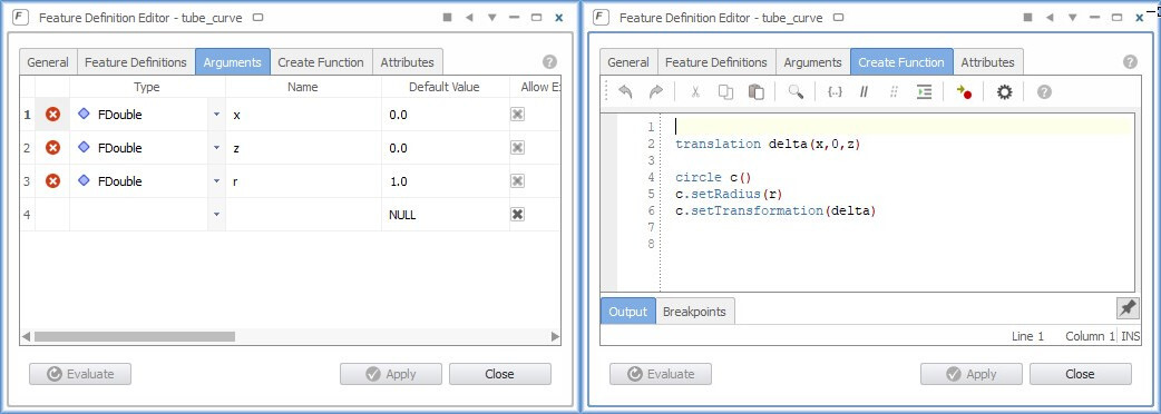
The first thing you need is the curve that you want to sweep. In this simple example, we define a parametric circle that has a radius value and a z‑location. The latter introduces the move into the 3D space. This custom curve definition is done within feature definitions. Features give you a generalized scripting environment to design any type of custom curve. The following picture shows the circle definition and its two input parameters called “z” and “r”:
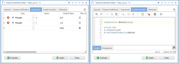
Curve definition with input parameters "z" and "r"
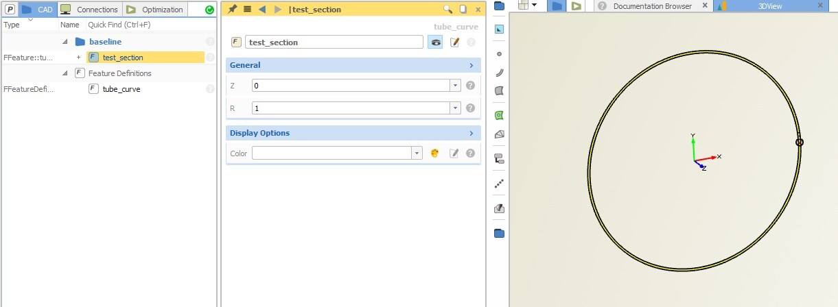
The circle is created in the XY-plane by default, and then translated in the z‑direction using the input z‑value. Such a command-based definition can be typed manually, or it can be generated interactively from a given curve in CAESES. We can test this curve in CAESES by creating a test section of the definition:
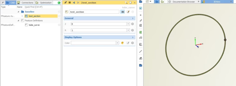
Test section curve with the two input arguments "z" and "r"
That’s it for the curve definition. You could now manually create a set of curves (e.g. 5 or 10) using copy & paste, change their radii and z‑values, and interpolate them by a NURBS surface to receive a tube. However, as we have learned in the last section, we want to automate this with meta surfaces. As a result, we will have less objects and a more flexible setup with the feature definition being one central place, where we can still modify our curve, if needed. Before we create the surface, we need to tell CAESES what the radii and z‑values look like when we sweep this circle definition.
Step 2: Functions for Input Parameters
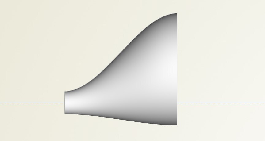
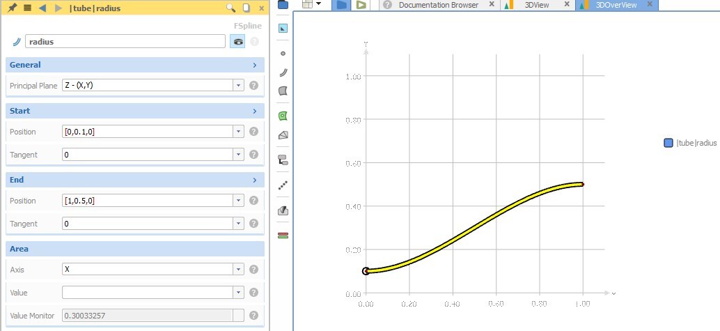
For the radius function graph, we can create a smooth 2D curve (a special f‑spline curve), and control the start and end ordinate values as well as the tangent angles. For instance, the tube start radius is r=0.1 and the end radius is r=0.5. We can define such a graph in the XY-plane and in the normalized interval [0,1]:
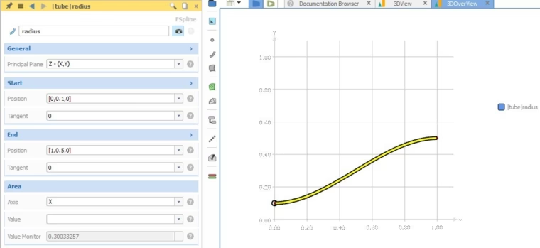
Tube radius function graph, defined in a normalized interval
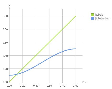
We also define how the input parameter “z” will develop during a sweep. This might seem a bit weird in the first stage, but “z” is also just another input parameter of the feature definition. In this example, the curve parameter “z” and hence the tube runs from z=0 to z=1 in the 3D space. We use a simple linear function for this sweep parameter, again in the same normalized system. As a result, we have the two function graphs, which define how the circle input parameters develop within a certain range:
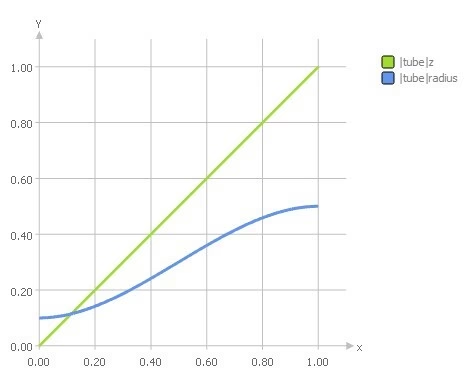
Function graphs for the two input parameters of the circle
Step 3: Connecting Curve Definition and Graphs
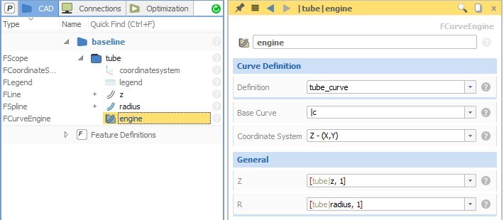
We need to connect the curve definition and the corresponding function graphs that describe the curve’s 3D behavior. For this purpose, there is the curve engine object in CAESES, where you choose the feature definition and where you set the function graphs:
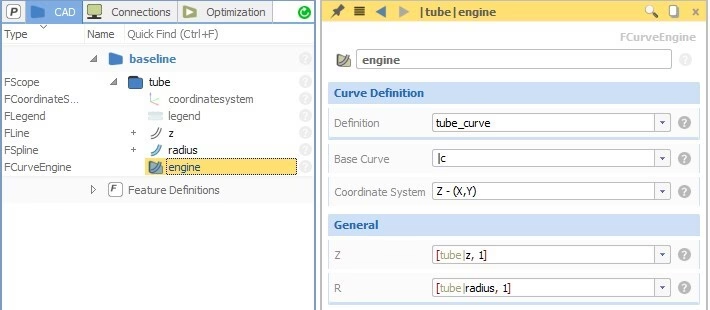
Connecting the circle definition with the function graphs
By the way: The name “curve engine” stems from the fact that, with the curve definition and the function graphs, you have all information available and connected to create a bunch of curves in the covered interval.
Step 4: Surface Creation with Meta Surface
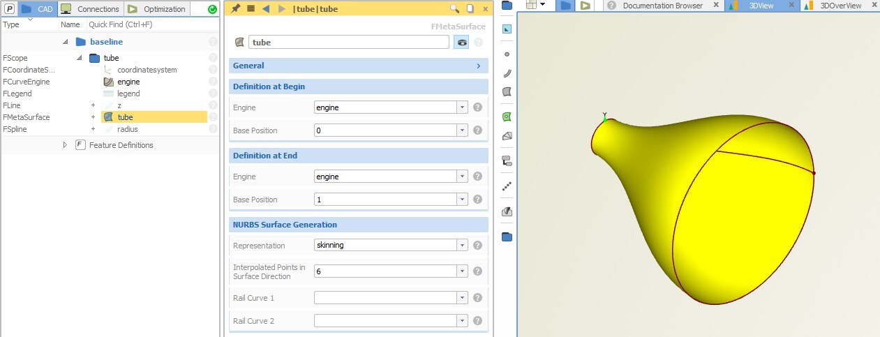
The final surface creation is done through the meta surface type. For this surface, you choose the curve engine from the previous step and a range (i.e., interval, called “base positions”), in which you want to create the surface. In our example, the function graphs are defined in the interval [0,1], so 0 an 1 are the base positions. The following picture shows a meta surface for the tube that is now based on the function graphs:
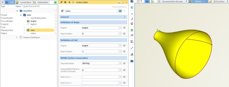
Meta surface based on curve engine and its function graphs
As an advanced feature, the meta surface allows you to set two different curve engines in order to blend from one curve definition to another (e.g. from a circle into a square etc.). This is essentially the reason why curve engines are separated, and not part of the meta surface object.
You can control how many cross-sections are considered for the internal skinning process. There is also the meta surface option to set rail curves while sweeping, e.g. for curve definitions that are not closed. This makes sure that existing boundary curves are exactly met, which is important when it comes to creating clean solid geometry.
Meta Surface: Summary
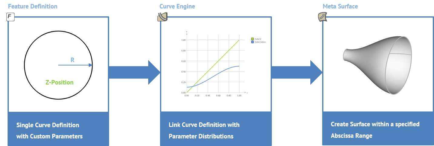
The entire meta surface process can now be summarized in the following stages:
- Curve definition with a set of parameters using feature definitions.
- Creation of function graphs for the single curve parameters.
- Linking of curve definition and function graphs by means of the curve engine.
- Creation of meta surface using the curve engine from step 3 within a specified interval.
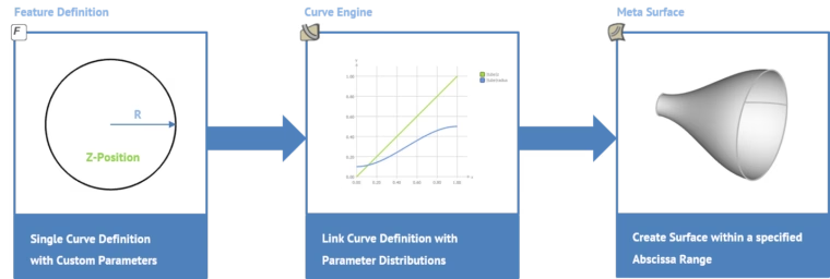
Extending the Parameterization
So far, this simple tube could also be quickly realized using a surface of revolution, and probably this would be the preferred way. However, we used this symmetric tube as an example to introduce the technical concept of meta surfaces. We have in mind the flexible design of more complex free-form surfaces, where meta surfaces can show their full potential. As a step into that direction, let’s make the shape asymmetric, also to get an idea of how easy it is to extend the existing parameterization.
One major benefit of this centralized curve definition is that we have only one place where to add new parameters. Say, we want to additionally translate the circle along the x‑axis while sweeping. All we have to do is to create another input argument “x” and slightly modify the feature definition code. That’s it — 10 seconds of work. By confirming this change, it will be applied to the existing model, i.e., the curve engine and the meta surface update automatically.
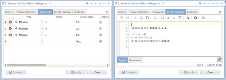
Add another input parameter to the curve definition to translate in x-direction
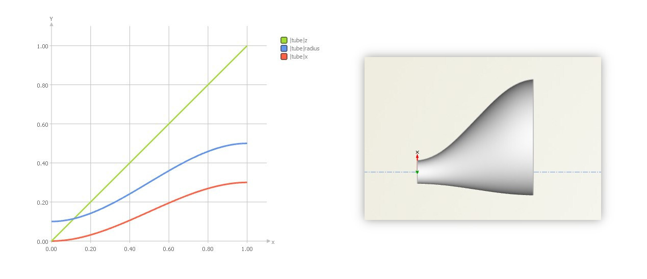
By using copy and paste, we can furthermore create another function graph for the x‑distribution and set it at the curve engine, in the same way as shown earlier for the radii distribution. This takes another 20 seconds of work and the result is shown below:
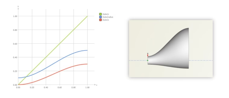
Asymmetric tube with extended parameterization and corresponding function graphs
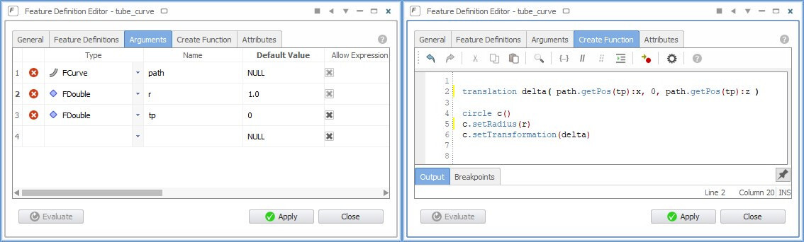
Just to trigger some ideas: As an alternative parameterization of this tube, one could use a 3D sweep path curve as input for the feature definition, so that e.g. “x” and “z” are picked from this path. Instead of having function graphs for these two parameters, we would then introduce a single curve parameter “tp” (any name works) to run on this path using a linear function graph in the curve interval [0,1].
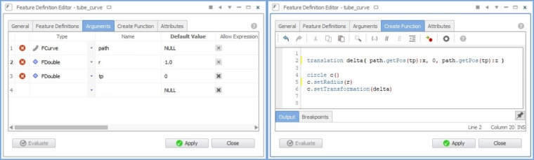
Alternative parameterization where the circle runs on a 3D path curve
More details and meta surface examples can be found in the documentation browser of CAESES. Basically, the point here is that you can grab information from anywhere in your CAESES project to create your custom curve definition for this advanced parametric sweep.
Automating Geometry Generation
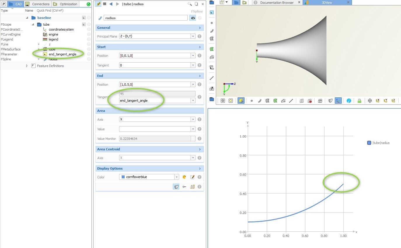
So, what to do with this now? The main purpose of meta surfaces is the efficient and parameter-reduced automated variation. CAESES allows you to create design variables with lower and upper bounds for any discrete value in your project setup. As a simple example, we could introduce a design variable for the end tangent value of the circle’s radii distribution:
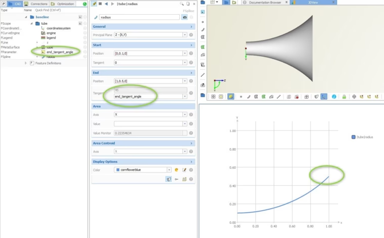
Introduce design variables for automated variation of the shape
Such a design variable is then controlled by the integrated optimization strategies or by external 3rd-party tools, such as ModeFRONTIER, HEEDS, OptiSLang and Optimus. You can also vary the start and end radii values, or you could create a completely different function graph (polynomials, interpolation curves, b‑splines etc.) and introduce design variables for coefficients, vertices and other discrete function values.
Meta Surface Applications
As mentioned in the introduction of this article, this is a generalized capability from which you can benefit no matter what application you work on. CAESES users create meta surfaces for complex shapes and if efficient controls are needed, particularly in automated processes. Let us look at a couple of applications:
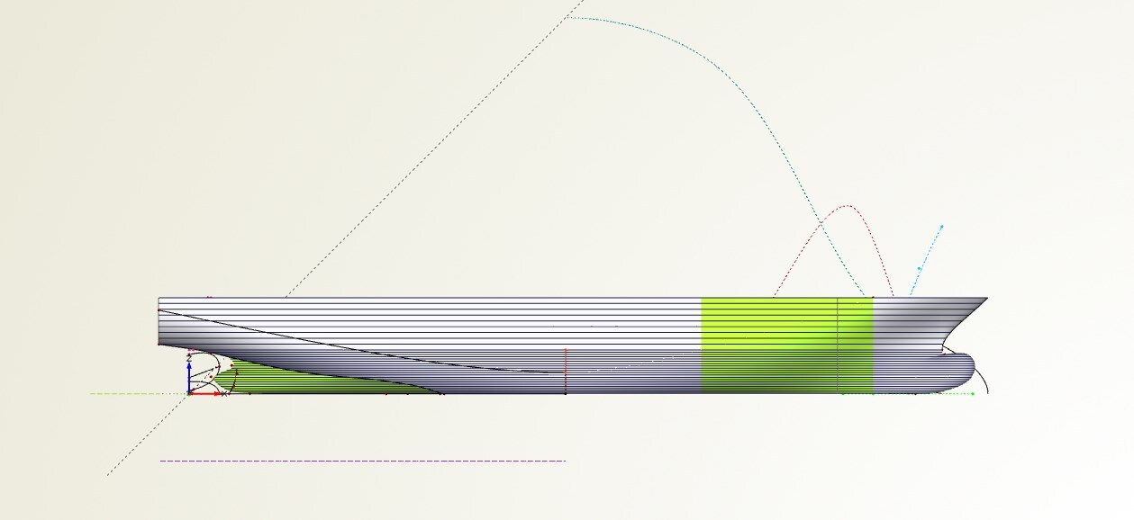
In the following animation, the meta surface of a ship hull is controlled by a set of function graphs for the ship’s displacement distribution, waterline tangent angles, beam and so forth. Note that with this technique only feasible hull geometries are created because the area constraint (which turns into the displacement) is already part of the user’s cross-section definition.
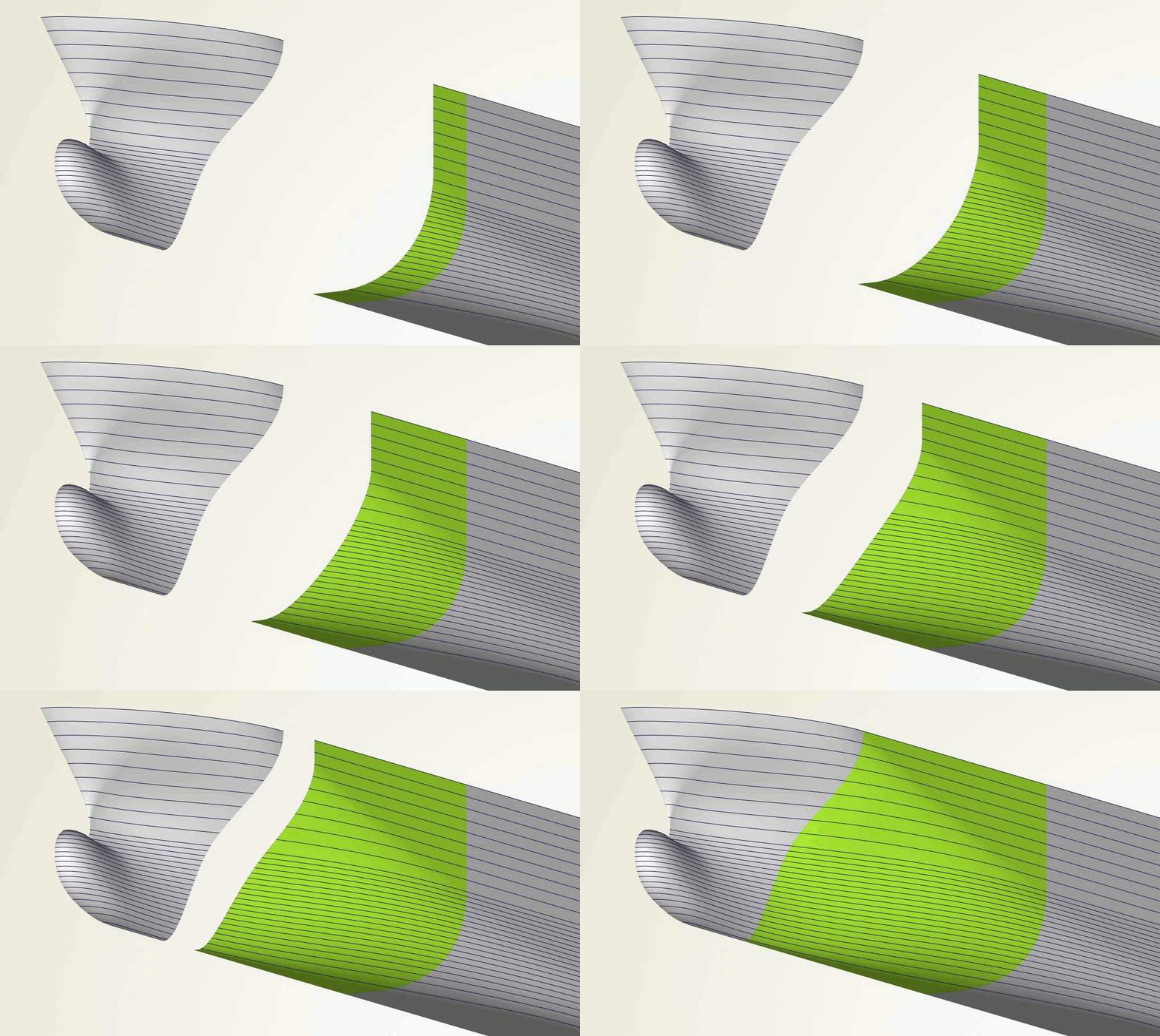
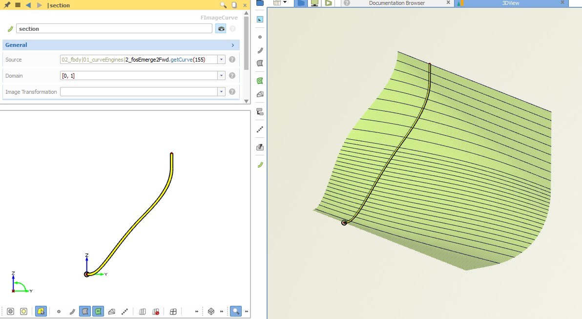
Since curve engines offer the option to obtain a curve at a certain location of the meta surface interval (i.e. where the function graphs are well-defined), we can visualize the curve at a specific location. You can use this capability to e.g. check and visualize single curves of the meta surface, or to obtain start and end curves of the meta surface.
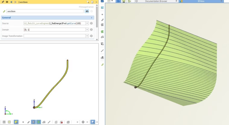
Parametric ship hull section at x=155 m, taken from the curve engine
For ship hulls, the function graphs are typically defined in a real-world coordinate system (e.g. [0, 200]), instead of using a normalized system. This has the advantage that function graphs can be visualized along the ship and hence directly correspond to the longitudinal positions. That makes it easier for the engineer to understand what’s happening in the model.
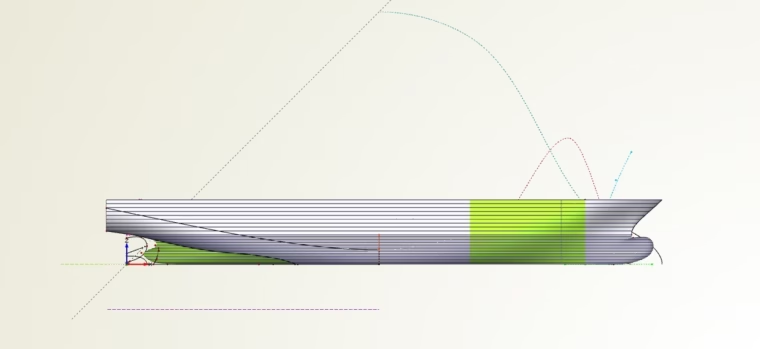
Ship hull with the function graphs for the meta surfaces
In the context of blade design for marine and turbomachinery applications, CAESES users define fully customized 2D profiles with any parameters for e.g. camber, thickness, leading edge radius, etc. For these single parameters, corresponding functions graphs define the span-wise or radial development of the shape. This allows engineers to have a higher control about their 3D blade shapes, for full customization in the context of exploring new innovative designs.
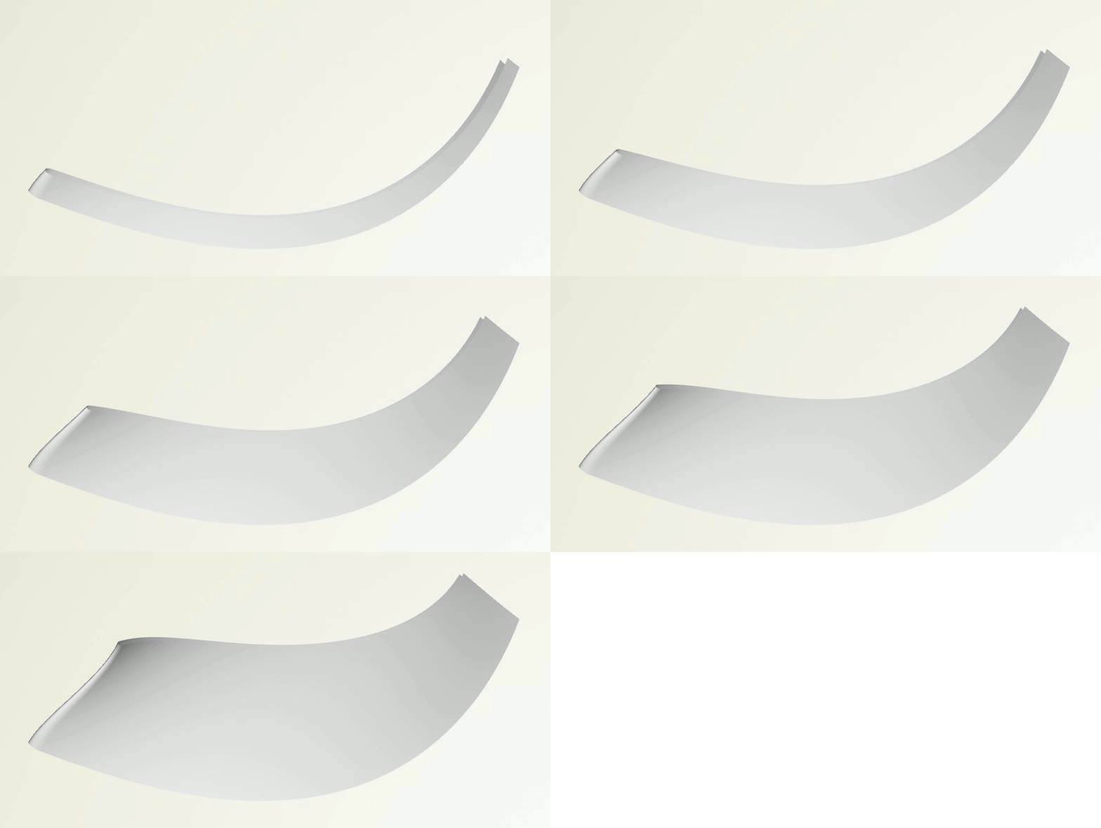
Meta surface for turbomachinery impeller blade
Another standard application for meta surfaces are volutes for pumps and turbochargers. The cross-section typically contains parameters for the A/R ratio, fillet radii and other geometry controls, for which function graphs are created, and varied during optimization runs — often in combination with the impeller, blade and diffusor meta surfaces.
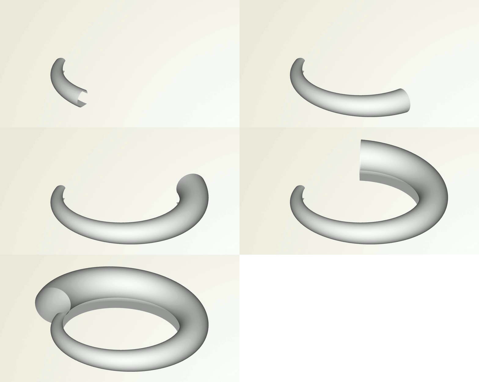
Compressor volute surface generation
In the automotive sector, there are a variety of components and parts that can be addressed with meta surfaces for shape optimization purposes. For instance, intake port designs can be controlled by function graphs for the cross-section area, while sweeping along a 3D path.
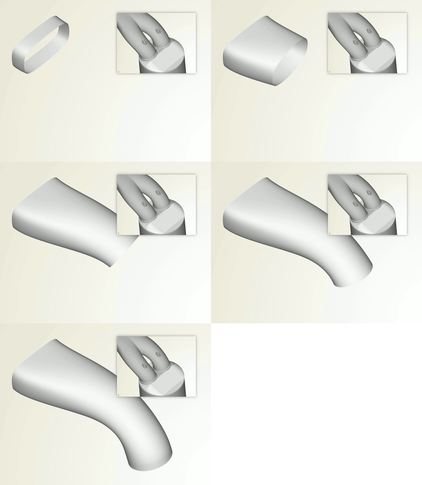
Intake port surface sweep along a path using function graphs for e.g. cross-section areas
More Information
Even though we put together a substantial amount of text for this article, the entire modeling process of e.g. the simple tube only takes 2 minutes in CAESES. With the curve engine and the meta surface capabilities, you obtain a flexible and ready-to-use parametric sweep process with literally unlimited possibilities! It might take some time and experimentation until you fully understand the power of this unique modeling offer. Note also that the custom curve does not need to be a 2D curve. Any curve definition that somehow moves into the space can be used as the base curve for the parametric sweep.
Check out the geometry modeling section of CAESES for more details about the entire CAD capabilities. More information about feature definitions and custom geometry can be found on the scripting pages.
Subscribe to the Newsletter
Are you interested in geometry-related topics and design optimization? Then stay tuned and sign up for our newsletter to receive short reads like this one!