Centrifugal Water Pump Design
by Johannes Weber
Centrifugal pumps are commonly used in industrial and residential applications due to their relatively simple design, manufacturing, and ease-of-maintenance. They are also rather efficient and easily applicable in different sizes. Thus, in the scope of his internship project at FRIENDSHIP SYSTEMS, Johannes Weber, a BSc student in Transport Systems Engineering at the Technical University of Berlin, was tasked with the implementation of a design process for a centrifugal water pump, making full use of the capabilities of CAESES.
Within this overarching aim, the individual project objectives were:
- Preliminary design parameter calculation for the radial impeller, based on the selected pump characteristics.
- Parametric modeling of the impeller.
- Flow domain modeling for CFD analysis.
- Dimensioning and modeling of the spiral casing, including the volute and the exit diffuser.
STEP 1 | Pump Type and Parameter Selection
A radial type impeller was selected and the B‑NM-50/200A/C pump from Linn-Pumpen GmbH [1] was chosen as a reference. The fundamental parameters of this pump are presented in the following table.
| Description | Symbol | Value |
|---|---|---|
| Volumetric Flow | Q | 78 m³/h |
| Pressure Head | H | 55 m |
| Speed | N | 2900 rpm |
With the help of the Buckingham-Pi-Theorem, the specific speed is defined as a non-dimensional parameter for turbomachines. However, in most cases in the industry the dimensional form of the specific speed is used. Consequently, the dimensional form was used in this project and calculated as Ns= 1091 (US) [2].
STEP 2 | Preliminary Pump Design
While CAESES has an extensive set of dedicated modeling functionality for turbomachinery, it does not provide preliminary design methodology out-of-the-box. However, the so-called feature scripting functionality provides the user with a complete programming environment that allows them to write their own custom routines. This approach was used here to implement the preliminary dimensioning of the pump based on selected empirical formulae and correlation diagrams.
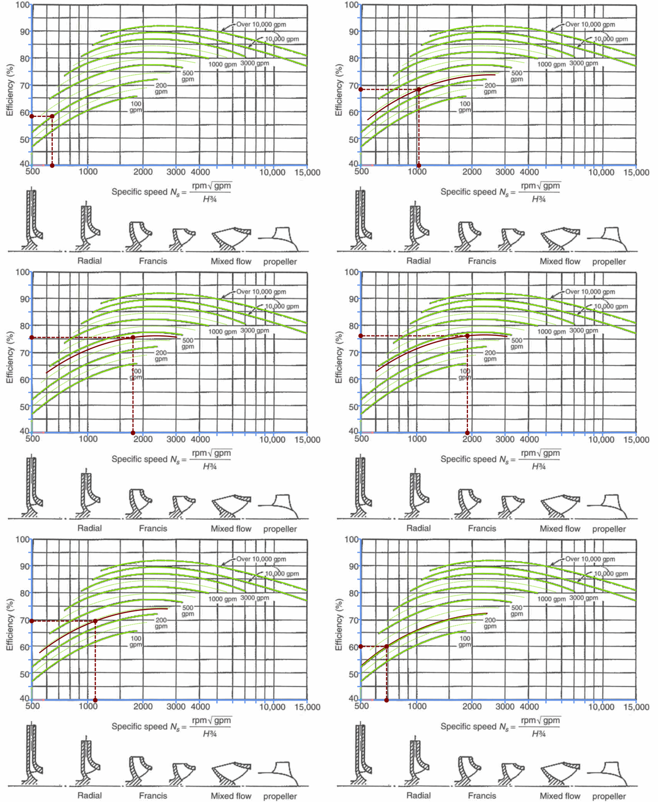
Determining Efficiency from Overall Efficiency – Specific Speed Diagram [2]
The calculation of the hub diameter was set up using the Overall Efficiency – Specific Speed [2] graph and the resulting shaft torque. The suction diameter, which is highly important for avoiding cavitation at the leading edge of the blades and accommodating the minimum-flow requirement, was determined keeping the cavitation criterion (NPSHR) in mind. For the calculation of both suction and impeller diameters, the Flow Coefficient – Specific Speed [3] graph was employed and implemented in CAESES.
Another important geometric design value is the minimum outlet width, which was calculated through the graph of Relative Outlet Width — Specific Speed [3] and applied in CAESES. Due to possible cavitation and flow separation at the blade, the minimum outlet width should be increased by a certain margin to guarantee the desired volumetric flow.
The calculated meridional dimensions of the impeller are given below.
| Description | Symbol | Value |
|---|---|---|
| Hub Diameter | Dh | 23.66 mm |
| Suction Diameter | D1 | 93.28 mm |
| Impeller Diameter | D2 | 224.86 mm |
| Outlet Width | b2 | 20 mm |
Further, determination of the leading and trailing edge blade angles is important to achieve the least amount of resistance. To calculate the appropriate values, the velocity triangles were used as a basis. The determined angles are presented in the following table, together with the calculated minimum number of blades [3, 4]:
| Description | Symbol | Value |
|---|---|---|
| Angle at leading edge (hub) | 28.66° | |
| Angle at leading edge (middle) | 18.49° | |
| Angle at leading edge (shroud) | 13.58° | |
| Angle at trailing edge (hub) | 25° | |
| Number of blades | 4 |
STEP 3 | Impeller Modeling
Using the previously determined main dimensions and geometric properties as input parameters, a full geometric model of the impeller was created. Obviously, throughout this process, the definition of several additional parameters that describe more detailed attributes of the geometry will be necessary. These parameters will introduce a sizable design space that can later be used to fine-tune and optimize the pump for its specific application using CFD, departing from the basic preliminary design.
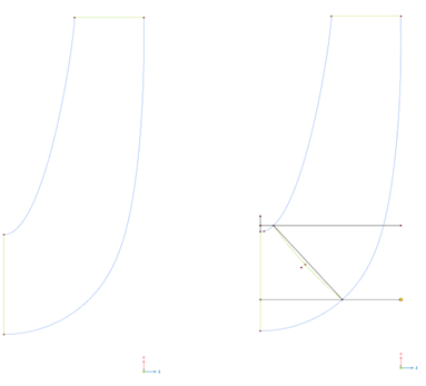
The first step in the modeling process of a radial impeller is to generate the 2D meridional contours. For this impeller, this was done by first defining a shroud contour that connects D1 and D2, taking into account the outlet thickness. The hub contour was then derived as an offset curve from the shroud with a given width distribution between the inlet and outlet width.
The leading edge, which serves as the stacking curve, was initialized as a simple straight connection of two points, located on hub and shroud contour, respectively. These points were each defined by the intersection of a given diameter and the corresponding contour and can be varied by two design variables. Subsequently, the possibility to create a curved leading edge was introduced using an intermediate interpolation point positioned at a parameterized normal distance to the initial straight leading edge.
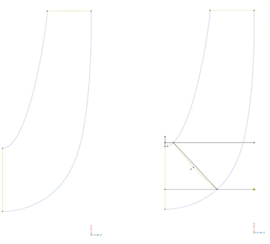
Meridional Contour Definition
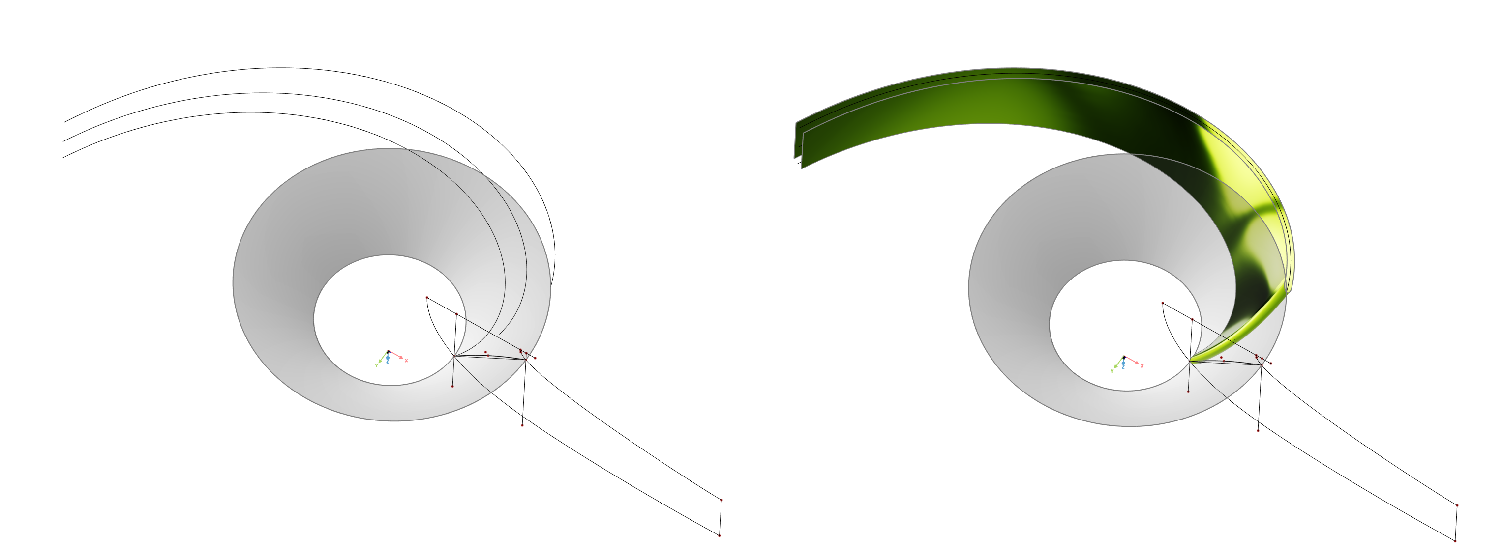
Camber lines at the hub, mid and shroud were created using a so-called Stream Section curve in CAESES, which is offered as pre-defined feature with the option to create the camber curve in different modes. The blade angle distributions used as an input to the camber line generation are defined in a separate diagram. Finally, the three camber lines are aligned at the trailing edge by rotating them with the difference between their individual wrap angle and the wrap angle from the hub camber line, resulting in a perpendicular trailing edge.
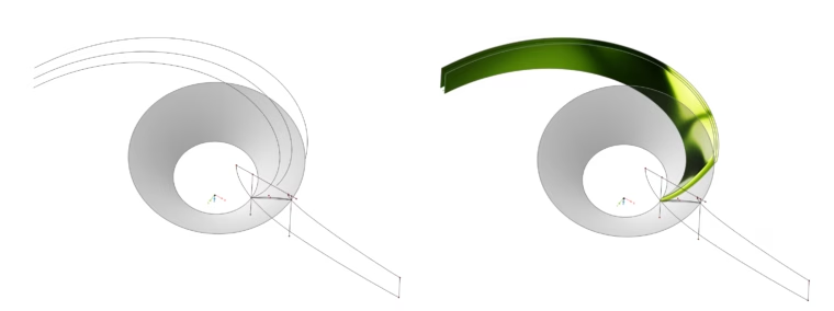
Blade Modeling
Then, the mean camber surface was modeled as a lofted surface interpolating the different camber lines, followed by the blade surface, which was created by applying thickness normal to the camber surface, again using a pre-defined section definition provided in CAESES and a specified thickness distribution.
Finally, the solid blade is the result of intersecting different surfaces to the desired closed boundary representation (Brep). The solid hub is defined in a similar way, connected to the blade with a Boolean operation an the root fillet is generated at the intersection.
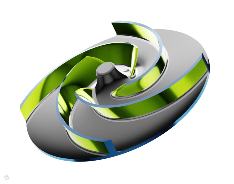
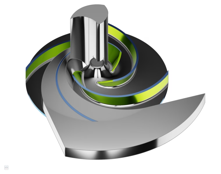
Impeller
As the preliminary design procedure is built directly into the parametric model of the pump, the complete model can simply be updated by changing one or more of the pump’s parameters. The impact of all three fundamental parameters (H, Q, and N) on the impeller geometry is visualized in the animations below, obtained by varying each parameter with a linear increase.
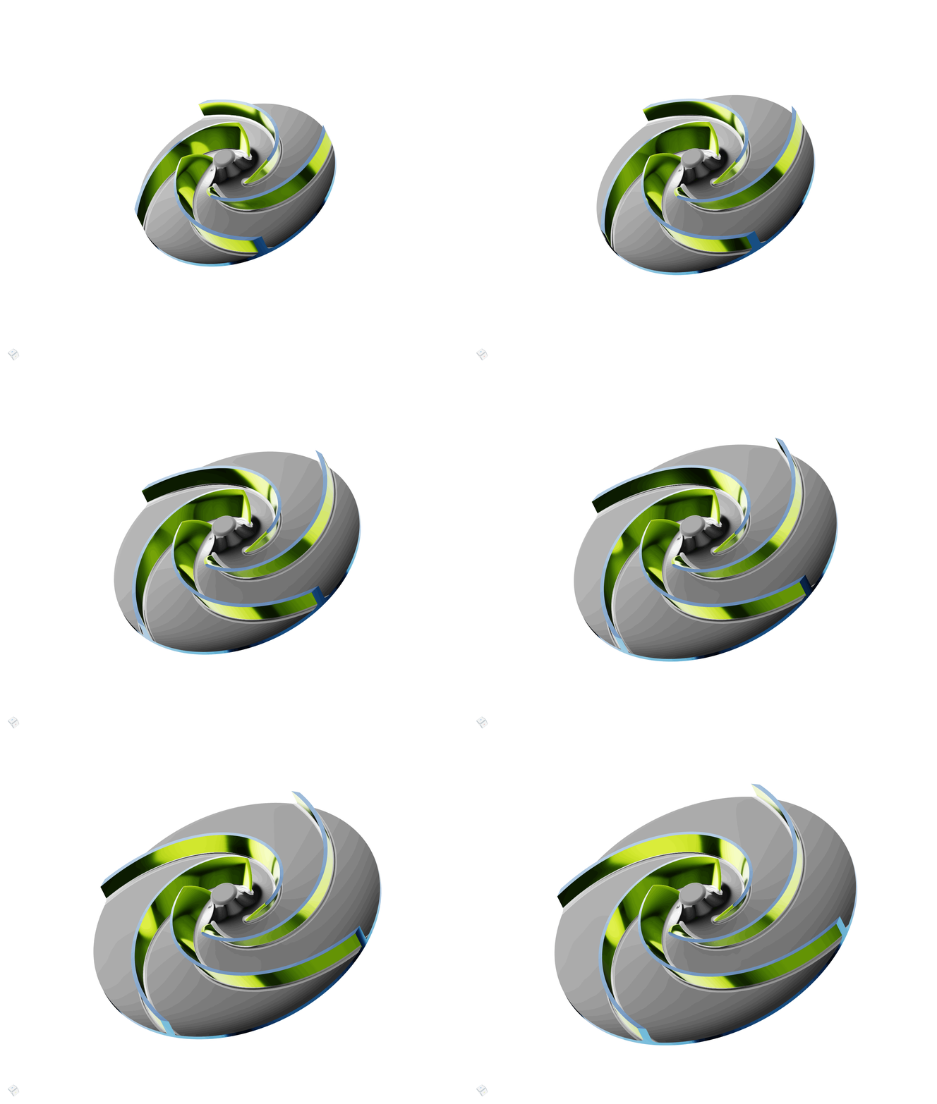
H = [40m , 100m] | With an increasing pressure head, the impeller diameter also increases
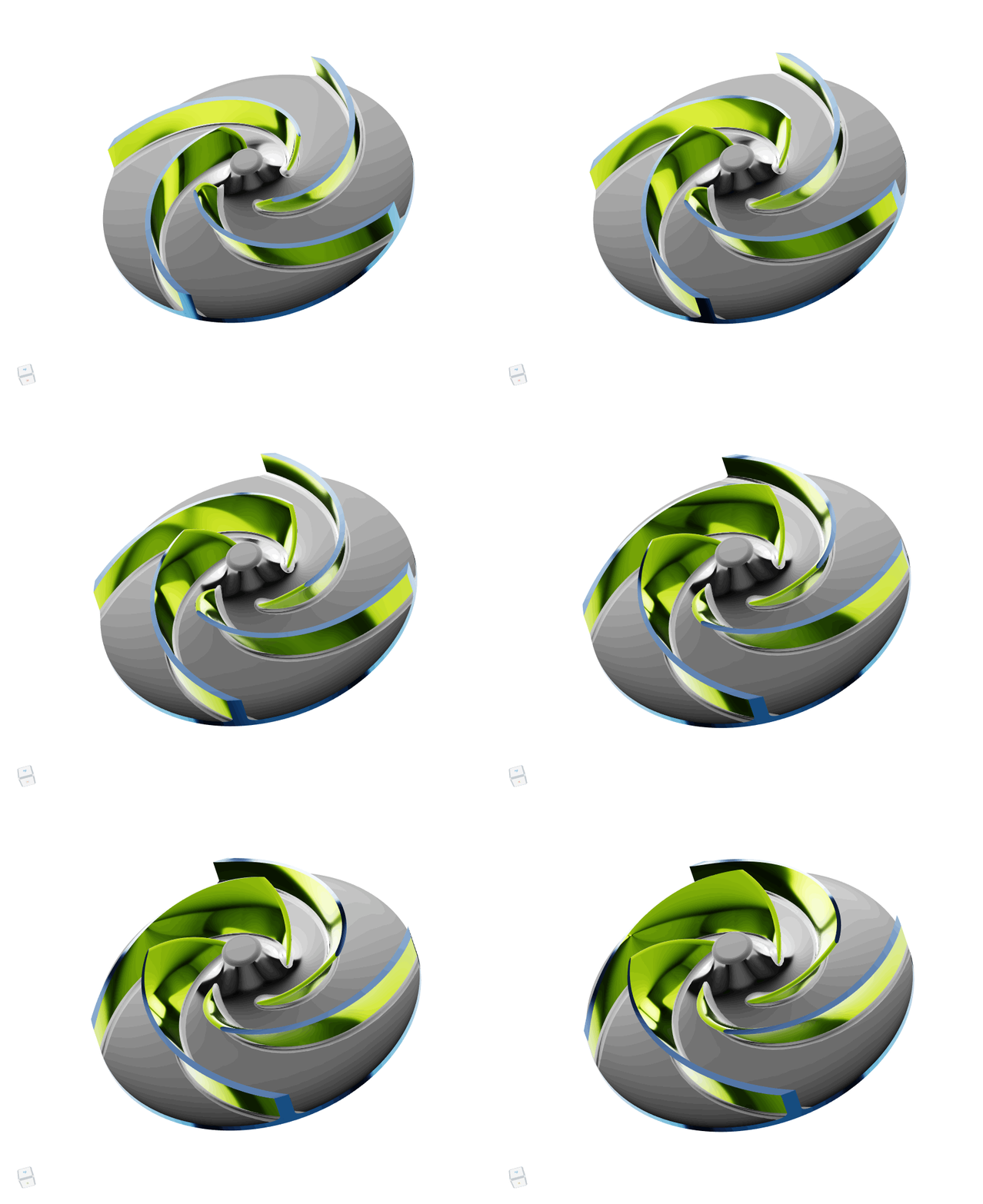
Q = [0.015 m3/s , 0.04 m3 m/s] | With the increase of volumetric flow rate, blade wrap and lean angle grow
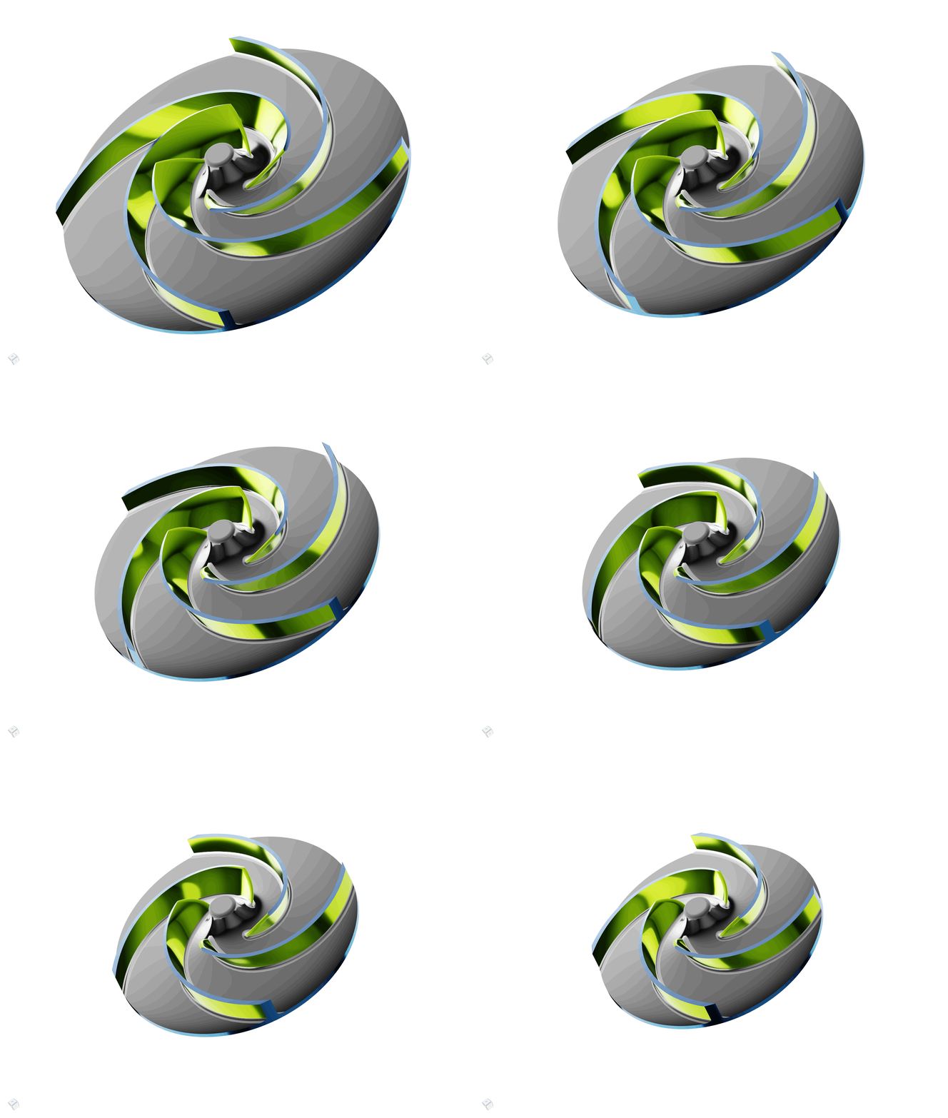
N = [1200 rpm, 3500 rpm] | When the speed increases, the impeller diameter decreases
STEP 4 | Flow Domain Modeling
The flow domain is the actual geometry that will be exported to an external grid generator for meshing and can either be modeled manually or using a selection of pre-defined feature definitions provided in CAESES. In this study, manual modeling was used to generate a periodic single blade passage domain, resulting in a robust definition that conforms to the respective changes of the impeller geometry.
Flow Domain
STEP 5 | Spiral Casing Modeling
The dimensions of the volute and the exit velocity were calculated by the method and graphs presented in the book „Fundamentals of Turbomachinery“ [2].
With these starting values at the volute exit, an algorithm can be started, which continuously determines the geometric values at each cross-sectional position. The result was an A/R ratio of ∼16.07 at the exit, whereas the starting A/R from this calculation was 0. [2]
Due to the disadvantages of manufacturing a volute with a starting A/R ratio of 0, it is common in the industry to maintain a constant A/R ratio in last part of the volute. In this project, a constant A/R ratio with a value of ∼1.49 was applied to the initial 5% of the volute’s total arc length.
After defining the dimensions, the volute together with the diffuser and the tongue surface in between the volute and the diffusor could be modeled. This was simply based on the CAESES tutorial „Volute Modeling“ and the included Feature Definitions. The final result of the spiral casing together with the radial impeller can be seen in the following image.
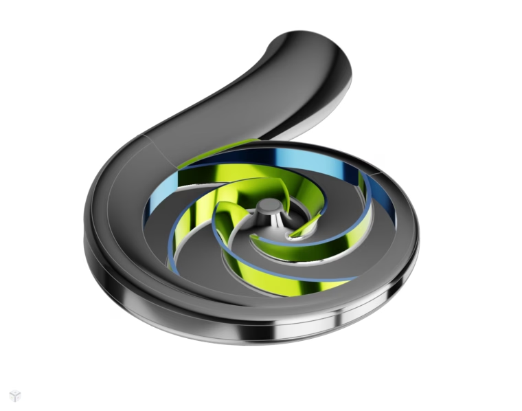
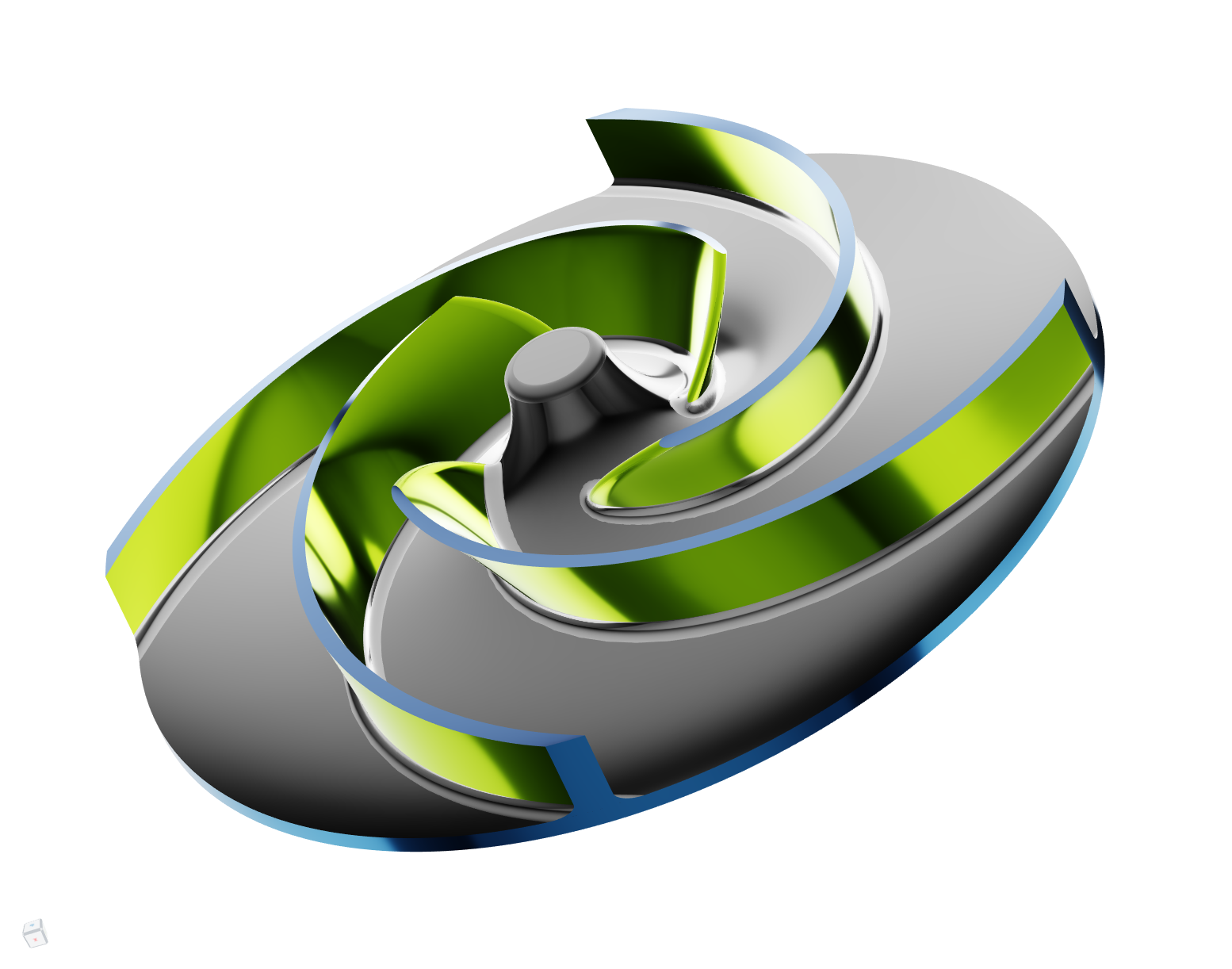
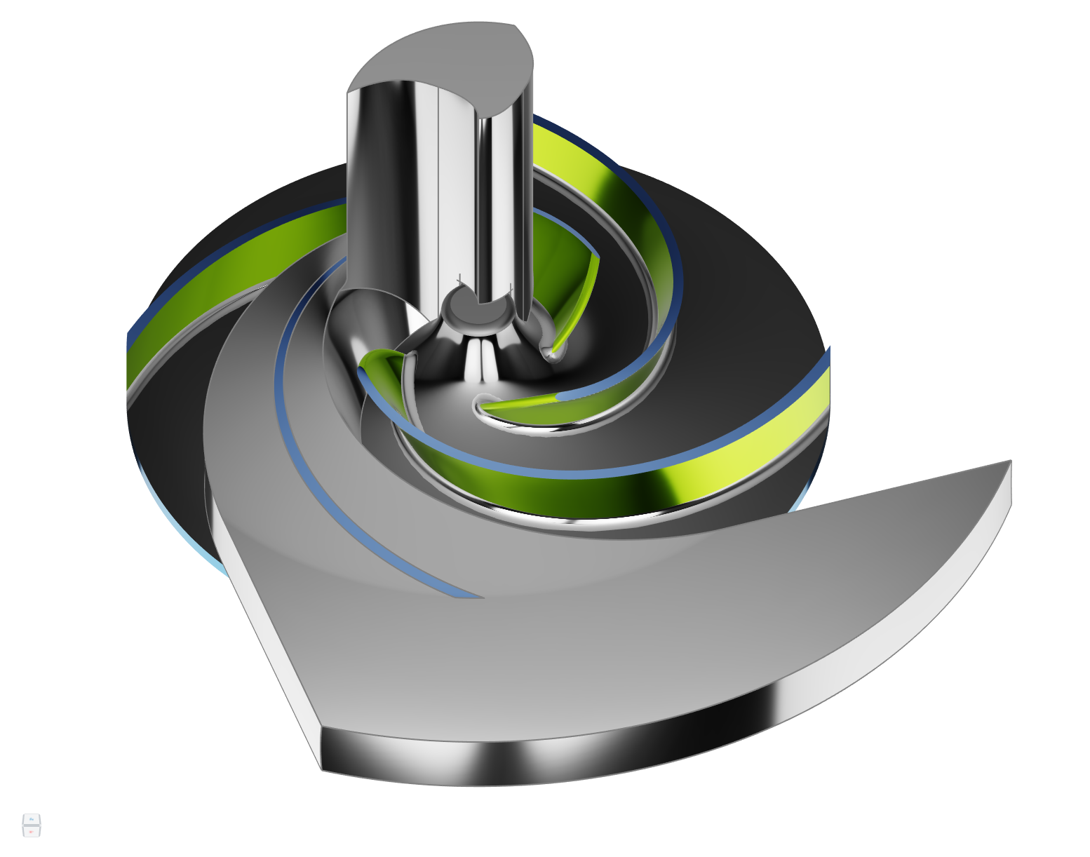
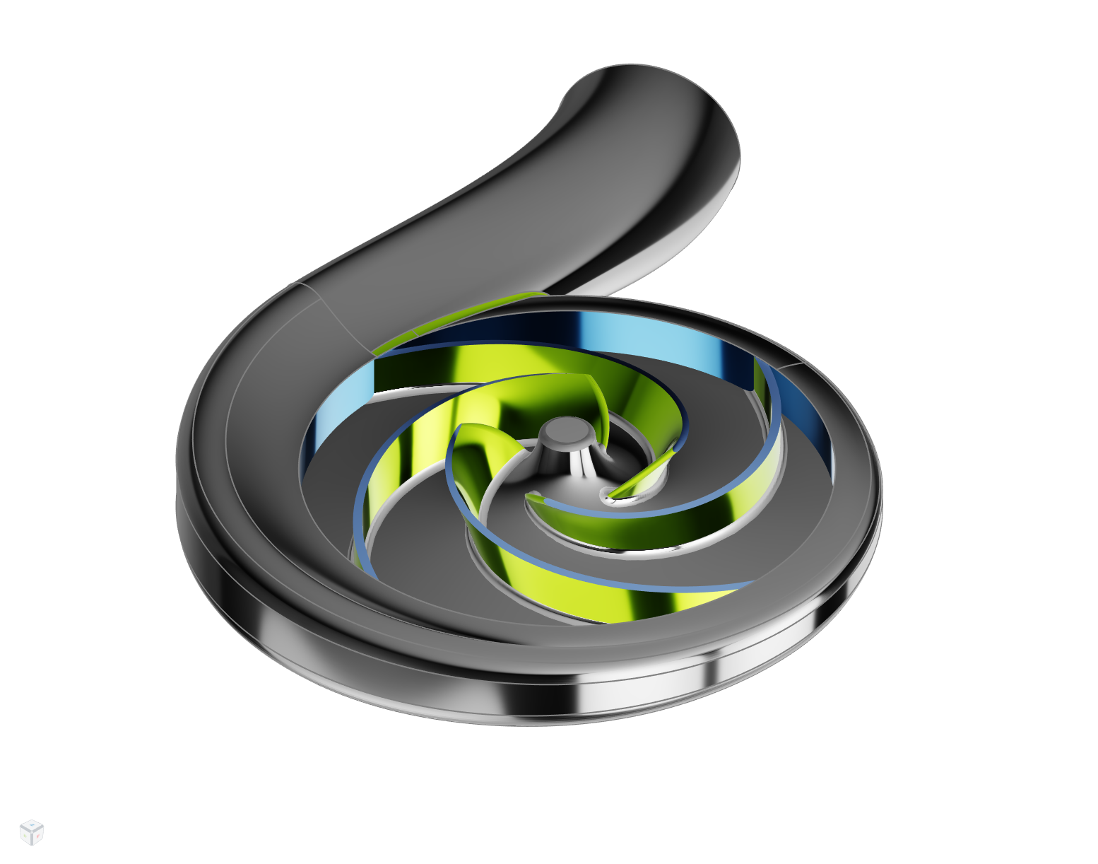
Spiral Casing and Impeller
Conclusion
By using CAESES, the evaluation of different values of the pump’s fundamental parameters is fast and practical. The calculation of preliminary design parameters, as well as empirical graphs, can be implemented directly into CAESES with the help of feature definitions, automatically resulting in a correct dimensioning of the radial impeller for the current parameter requirements. This makes it easy to use the project for preliminary design development.
Another aspect is the possibility to integrate a virtually unlimited — and fully customized — selection of additional parameters that allows to fine-tune every aspect of the geometry, creating an ideal set up for a quick variation of the shape after the preliminary design in order to optimize the pump on the basis of flow analysis.
About the Author
Johannes Weber is a Transport Systems Engineering student at the Technical University of Berlin. He conducted his internship at FRIENDSHIP SYSTEMS in 2022.

“The process of first getting in touch with CAESES was a great experience due to the range of tutorials, which made the learning process straightforward and transparent. Because of the endless capabilities of creating, adjusting, and optimizing geometric models, it made the process of designing the radial pump and implementing the calculations fast, efficient, and reliable. In combination with a modern interface, for me, this is a state-of-the-art software, which I am looking forward to use and work with in the future.”
Johannes Weber
BSc Student
References
[1] LINN PUMPEN, publ., 2015: Close Coupled Centrifugal Pumps with flanged connections. [Last checked on: 30.05.2022]. Available via: https://www.linn-pumpen.de/com/centrifugal-pumps/NM-MNS-DIN-pumps.html
[2] PENG, W. W., 2008: Fundamentals of Turbomachinery. 1st Edition. Hoboken, John Wiley & Sons, ISBN 978 – 94-017‑9627‑9
[3] GÜLICH, J. F., 2020: Kreiselpumpen – Handbuch für Entwicklung, Anlageplanung und Betrieb., 5th Edition. Berlin, Springer Viewig, ISBN 978 – 3‑662 – 59784
[4] CFturbo, publ., 2021: User manual for CFTurbo Software, Dresden [Last checked on: 30.05.2022]. Available via: https://manual.cfturbo.com/CFturbo_en.pdf
More Information
See this overview to learn more about the capabilities of CAESES for turbomachinery design and contact us to discuss your individual requirements and our solutions in more detail.