Automated Optimization using Adjoint Flow Solvers
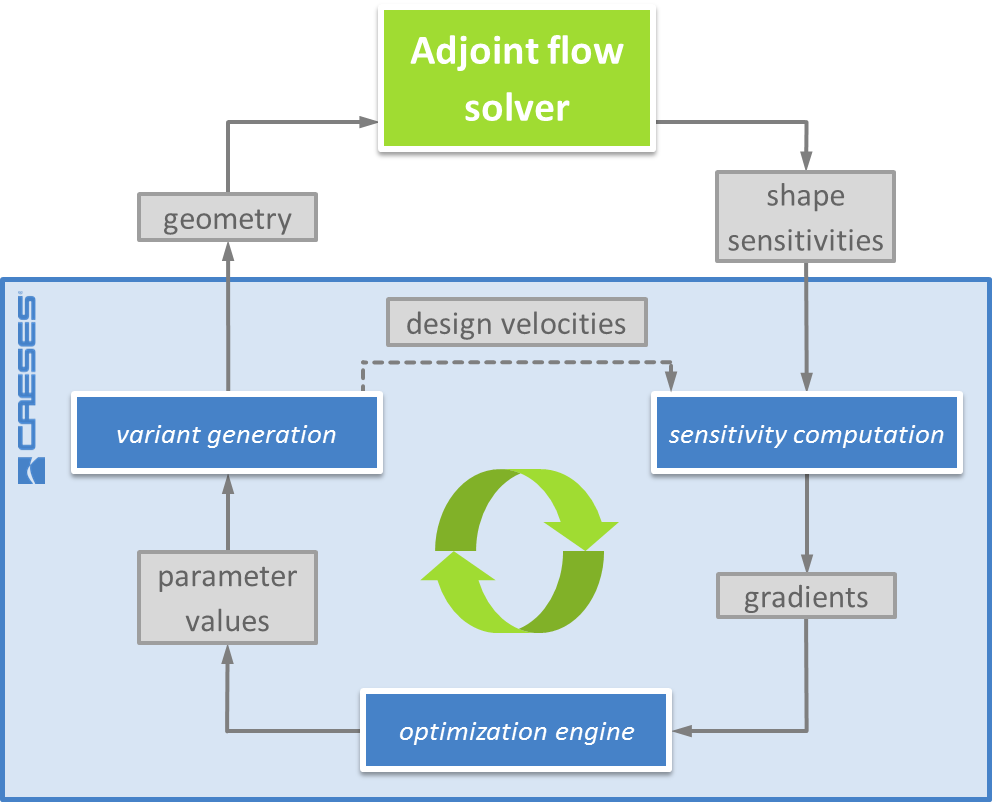
Here at FRIENDSHIP SYSTEMS, we recently carried out a case study for an automated optimization process based on the shape sensitivities computed by an adjoint CFD solver. The open-source optimization toolkit Dakota by Sandia National Labs, that is integrated in CAESES® through a direct interface, provided an optimization strategy that can directly receive the gradient information obtained from coupling adjoint shape sensitivities to CAD model parameters as input (check out this recent article). Based on this information, the algorithm selects the parameter combination for the next variant that is then created by CAESES® and analyzed by the adjoint flow solver.
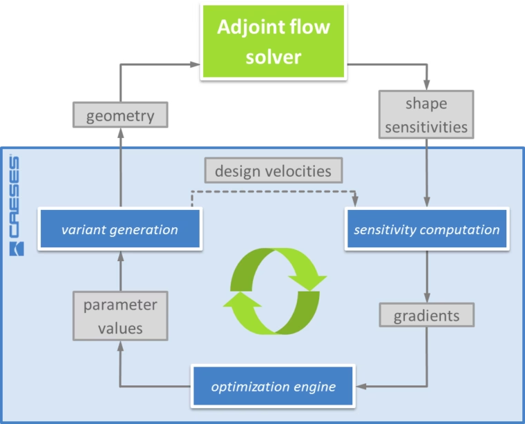
Process diagram for automated optimization using gradient information from adjoint analysis
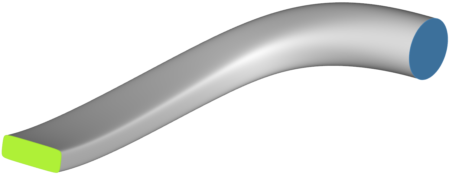
The geometry considered in this study was a simple fictional duct with a 90-degree bend that could resemble a component taken from an internal combustion engine. Inlet and outlet were fixed in position, shape and orientation, but everything in between was free to change. The geometry was modeled using an intelligent variable surface design in streamwise direction and 13 defining parameters that control the shape of the duct’s path and cross-section. The geometry was transferred using a “colored” STEP format that allows transferring patch names.
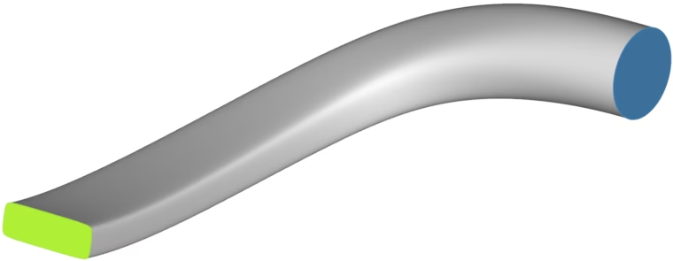
Geometry model of the duct including unique identifiers for the inlet and outlet patches
The flow solver STAR-CCM+ was used to solve the primal and adjoint equations for every variant. The fluid was air with an inlet velocity of 50m/s, which corresponds to a common gas velocity in engine parts. The overall computation time, including the meshing with about 33.000 cells, was about 6 minutes. The surface shape sensitivities were calculated by STAR-CCM+ after the adjoint simulation was completed and exported in Ensight Gold format, to be able to import this information to CAESES®. From within CAESES®, the STAR-CCM+ calculations were triggered and controlled with JAVA macros. The overall pressure drop was used as the objective function.
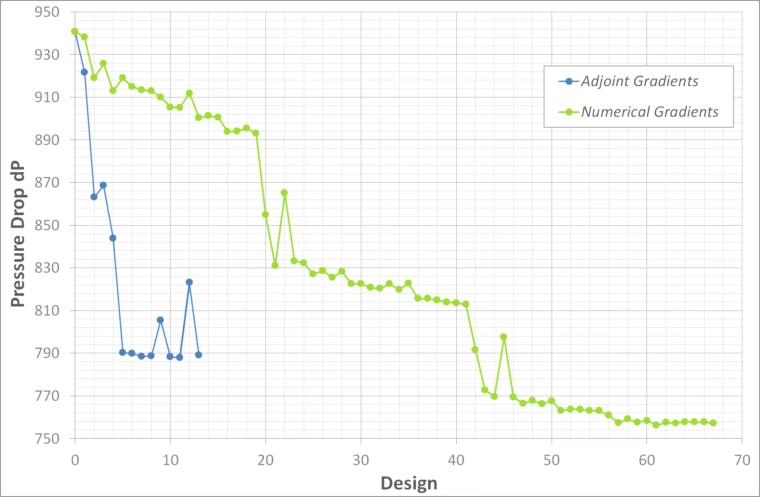
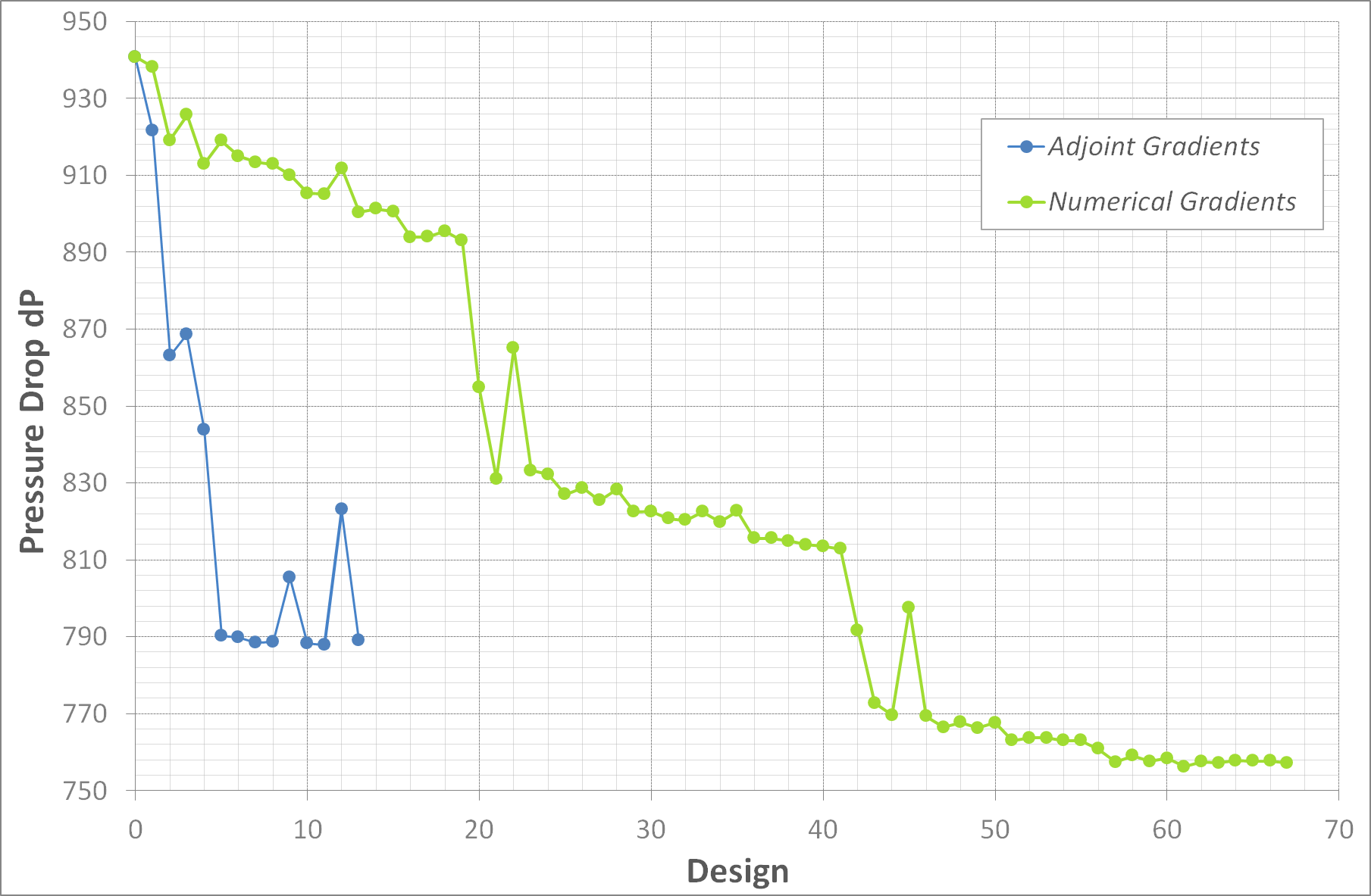
Convergence plot for the pressure drop from the automated optimization with and without gradient information from the adjoint CFD computations
13 geometry variants were analyzed in the course of the automated optimization, whereby a local minimum with a 16% improvement of the objective function was already found after a very quick descent at the 5th variant, after which no significant improvement happened any more. A conventional optimization with a standard deterministic algorithm was carried out for comparison purposes. Although this lead to a slightly better local minimum (approximately 20% improvement), it required a significantly higher number of variants, and therefore function evaluations (67 new designs). Especially apparent are the small steps during the exploration phase of the algorithm that are required for the numerical determination of the local gradient direction. Obviously, this step is omitted when using the gradient information from the adjoint analysis, which is crucial for the potential time saving of this optimization approach.
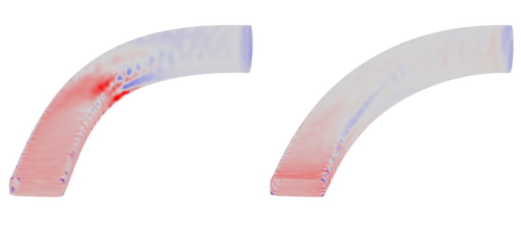
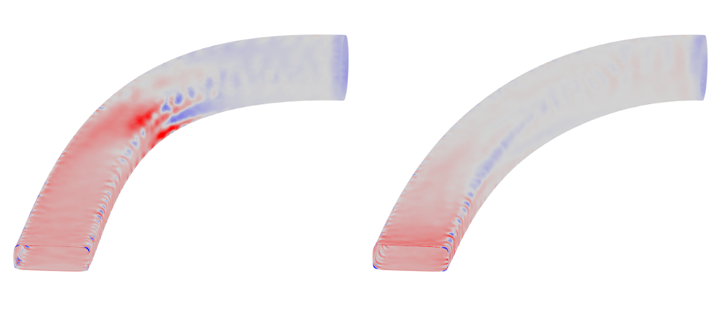
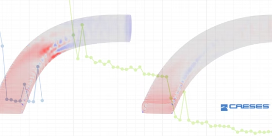
Shape sensitivities for initial (left) and optimized design (right)
The convergence of the design can also be very well observed in the difference of the shape sensitivity plots between initial and optimized design. The shape sensitivity in most parts of the geometry has been reduced to almost 0, except for the areas where the modification of the geometry was constrained by the fixed inlet and outlet geometries.
Summary
Using adjoint shape sensitivities and coupling them to the CAD model parameters in the context of optimization allows for a significant speed up of the convergence process and an optimized geometry that can directly be fed into the downstream CAD design process. Additionally, since the expenses do not scale with the number of parameters, all form parameters of the model can be involved into an optimization, without having to do a pre-selection. One must consider, however, that the predictions based on the adjoint sensitivities are only valid for small (in strict mathematical sense infinitesimal) changes to the geometry and that using this information for optimization is a local procedure. If a global optimum is searched, one might still have to precede the actual optimization by a Design of Experiments (e.g. using random sampling algorithms such as the Latin Hypercube Sampling) to scan the wider design space.
More Information
If you are interested in fast and automated shape optimization using adjoint information, then simply get in touch with us. We look forward to discussing it with you in the context of your individual engineering application. More information about using Dakota together with CAESES® can be found in this recent blog post about response surface methods.
Follow Us
Are you interested in CFD-driven design optimization? Then stay tuned and sign up for our newsletter to receive short reads like this one here! Don’t worry, we won’t bother you with too many emails. Of course, you can unsubscribe at any time :-)