Direct Coupling of Parametric CAD and Adjoint CFD
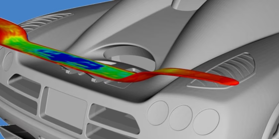
In the context of different R&D projects over the last few years, we at FRIENDSHIP SYSTEMS have developed and implemented a new method for our product CAESES® that is based on the direct coupling of our efficient CAD parameterization and adjoint CFD computations. The main advantages of this method are:
- The largest possible design space can be considered for optimization. All parameters in the model can be involved, without the need for the user to understand the effect of each parameter.
- The effort does not scale with the number of parameters!
- No mesh morphing as in other CAD-free optimization solutions based on adjoint CFD. The CAD model is modified directly.
- The optimized geometry can directly be used in downstream CAD without re-modeling!
- Geometry constraints can be easily monitored and fulfilled!
- The local gradient of the objective function is computed directly. It can be fed into the optimization algorithm for faster convergence.
Introduction
Using parametric modelling in the design process allows for an efficient variation of the geometry. The total number of shape-defining parameters for a typical parametric model of a flow-exposed geometry (like a ship hull, turbomachinery or engine component) in CAESES®, however, can typically reach the range of 20 to 50. This means that for complex free-form geometries the number of degrees of freedom is still so large that, when using a direct optimization approach, taking into account all parameters, a high number of function evaluations, i.e., CFD computations, would be required to identify trends with respect to the necessary geometry modifications leading to an improvement of the considered objective function(s). Because of the long computation times, this approach becomes infeasible, especially when dealing with complex flow situations. In order to adapt the expenses to the available resources, the design engineer would typically select a suitable subset of parameters, either based on his experience or his technical intuition. Besides the disadvantage of reducing the available design space for the optimization, the selection of this parameter subset is often difficult, since the effect on the objective function is not known a priori. This is especially true when the engineer does not have enough experience to make a meaningful selection or when the model was produced by someone else, introducing the additional uncertainty of the specific impact of every parameter on the geometry.
Adjoint CFD
The decisive information for the flow optimization of a given geometry is the correlation between the objective function J and the form parameters αi. This correlation can be mathematically expressed through the so-called sensitivities – the rate of change (i.e., the gradient) of the objective when varying the form parameters. The individual sensitivities can be approximated by the finite difference quotient, which for n parameters in a classical gradient based optimization approach would require n+1 CFD computations to evaluate the corresponding modified geometry for every form parameter. As mentioned above, this direct approach is therefore not really applicable for a high number of parameters and expensive simulations. Of course, intelligent DoE strategies can possibly reduce the number of function evaluations, but they still significantly scale with the number of free parameters.
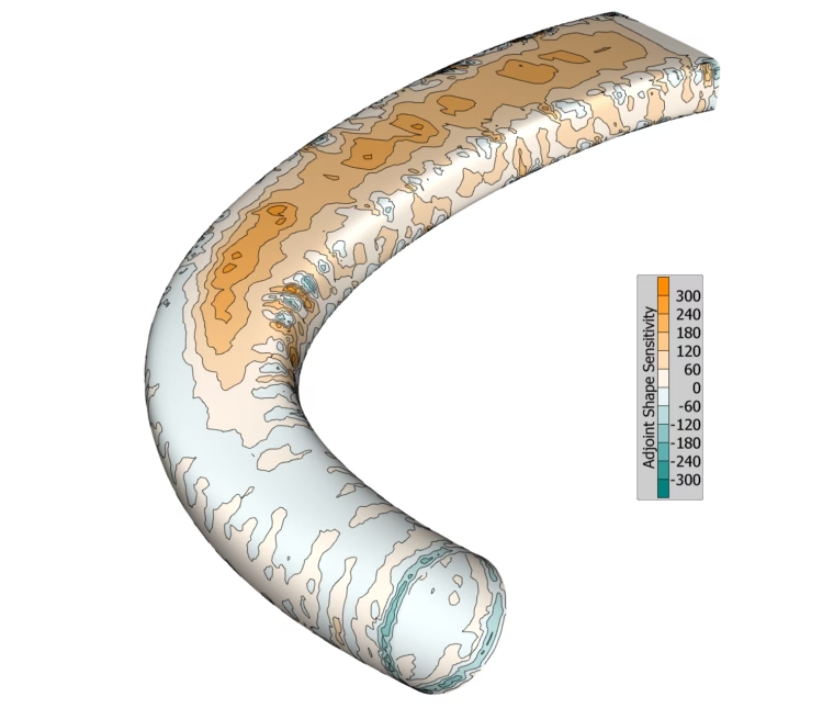
Visualization of shape sensitivities
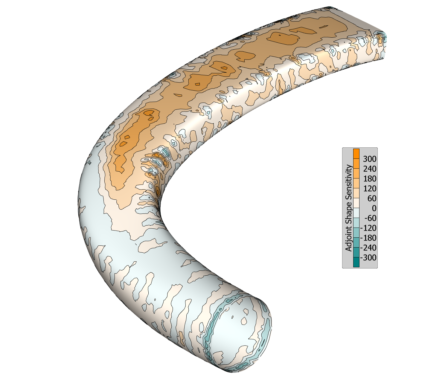
So-called adjoint methods, however, go the reverse way. Instead of evaluating the change in objective function due to a variation of parameter value, the required variation of the parameter values for a desired change in objective function is computed. Within a single computation, the adjoint method will yield the full gradient of the objective function, irrespectively of the number of parameters. The full analysis would require a conventional (primal) CFD computation, followed by one adjoint computation for each considered objective. In the context of shape optimization, the adjoint analysis will provide the so-called shape sensitivity as a result. This is given as field information on the surface of the model and describes the change of objective function due to normal displacement of the surface cells (∂J/∂nk). A positive value of the shape sensitivity indicates a local displacement in positive normal direction and vice-versa. The sensitivity is given by the adjoint analysis with respect to the CFD discretization of the model surface. For industry-relevant cases, the CFD geometry is typically described by ten thousands of nodes, and therefore degrees of freedom, so that the obtained sensitivity is described with a very high degree of detail, in a quasi-continuous way. In a CAD-free approach, this information can be directly used for a displacement of the grid nodes and, therefore, a deformation of the initial geometry. When using this approach, however, a disadvantage is given by the fact that the shape modifications are difficult to feed back into the design process and geometrical constraints (e.g. due to production restrictions) can be violated. This leads to the motivation of developing a method that maps these initial sensitivities for the degrees of freedom of the CFD geometry to the corresponding sensitivities ∂J/∂αi (rate of change of the objective function due to change of parameter values) of the CAD model parameters.
Mapping Adjoint Shape Sensitivities to the CAD Model Parameters
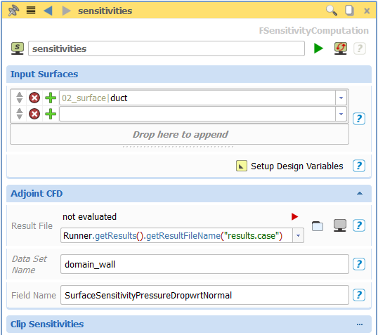
In order to map the adjoint shape sensitivities to the CAD model parameters, a new object – the Sensitivity Computation – that takes care of all the necessary steps, was implemented into CAESES®. Inputs to this object are the surfaces and the adjoint CFD results. Here is a screenshot:
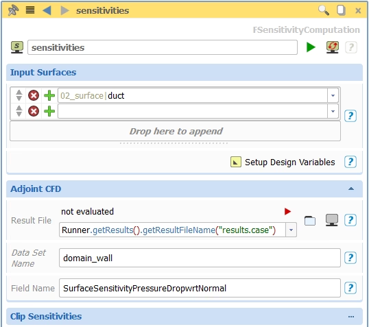
User interface of the sensitivity computation in CAESES
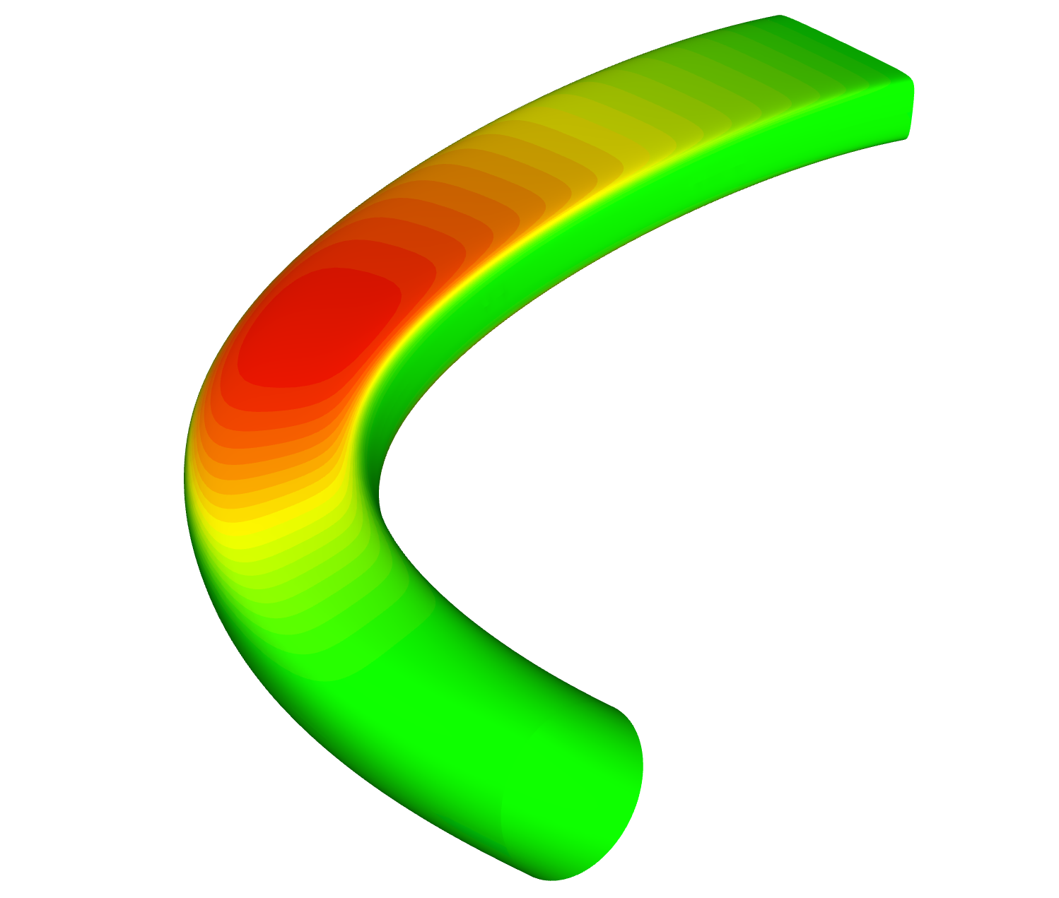
Initially, the adjoint sensitivities are interpolated from the CFD discretisation to the surface tessellation of the CAD model. Then, the local normal displacement of the model surface due to parameter variation – ∂nk/∂αi, the so-called design velocity – has to be determined. By tracking the dependencies for all model surfaces selected for this operation, all influencing parameters are automatically determined. These are perturbed by an individual amount related to a specified absolute displacement of the model surface in positive and negative direction and the normal displacements of the surface tessellation nodes are evaluated. For each element, the gradient ∂nk/∂αi can then be computed from the displacement due to the perturbation. Like the adjoint shape sensitivity ∂J/∂nk, this data can be visualized as a plot on the model surface.
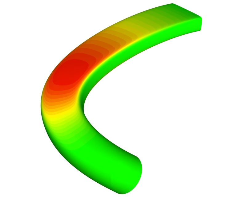
Design velocities: Visualization of the parameter effects
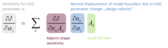
By comparing the two plots, one can already get a more or less good visual estimation about which parameters influence areas with high shape sensitivity and, therefore, have a more pronounced impact of the objective function. A more precise statement can be obtained by creating the product of ∂J/∂nk and ∂nk/∂αi for every tessellation element, weighting it with the local area, creating the sum over the surface and thereby computing the sensitivity ∂J/∂αi for every parameter.
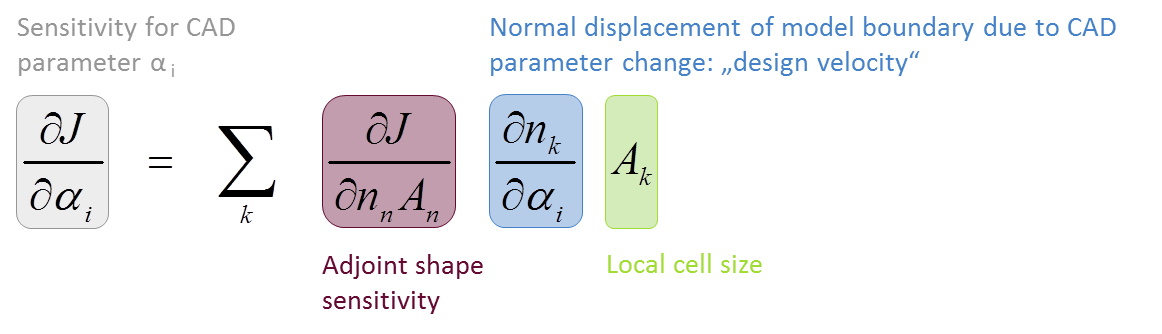
These scalar values for all involved parameters are collected and displayed in a table. They show the user which of the parameters have the biggest influence on the objective function and in which direction they should be changed in order to have a positive influence on the objective. This gradient information can be used to select a subset of the most influential parameters, as well as for a subsequent automated optimization process. In the former case, the parameter values can be manually changed or involved in a conventional optimization. In the latter case, the gradient information can directly be used by a suitable optimization algorithm to determine the search direction towards the (nearest local) optimum. This significantly speeds up the convergence, because the gradient does not have to be determined by the optimization algorithm in a numerical way.
More Information
This text is part of the paper “Direct Coupling of Parametric CAD and Adjoint CFD for the Efficient Optimization of Flow Geometries”. It additionally includes detailed case studies including pictures and diagrams for the optimization of an automotive rear wing, a ship hull and a duct. Gradient-based optimization strategies are also considered for finally having a fully automated design process. Follow-Up Article Check out our follow-up article optimization using adjoint flow analysis which describes this automation procedure by means of a duct example. If you are interested in the full article, just get in touch with us.