Poly­curve and Surface Splitting

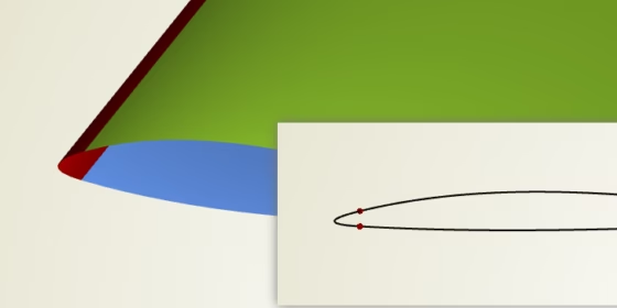
The poly­curve type in CAESES® is some­thing that gets used quite a lot, in par­tic­u­lar in the context of surface gen­er­a­tion through the meta surface tech­nol­ogy where you need to have a single curve def­i­n­i­tion. The poly­curve simply takes a set of N curves and rep­re­sents a single curve with an own curve domain based on this input. Curve domains typ­i­cally run in the interval [0,1]. The inter­est­ing thing is that the curve domain is then defined accord­ing to the number of input curves.

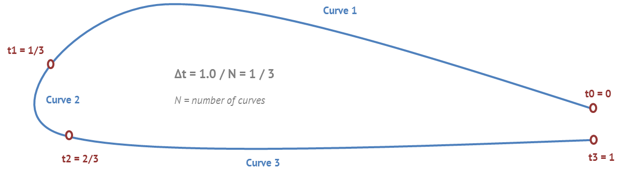
See the fol­low­ing illustration:

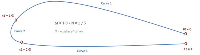
Let’s assume you want to get the exact end position of the first input curve. For N=3 input curves of a poly­curve, the poly­curve para­me­ter is simply t1=1/3. The con­nect­ing para­me­ter loca­tions are defined by t_​i = i * 1 / N where N is the number of input curves, and i runs from 1 to N‑1.

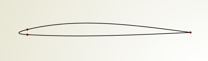
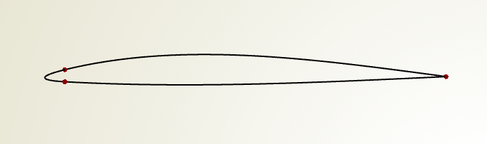
Here is an example where the screen­shots are taken from CAESES®. A simple profile gets modeled which runs from the trailing edge (right-hand side) via the leading edge back to the trailing edge. Three curves are gen­er­ated sep­a­rately and then put into a polycurve:

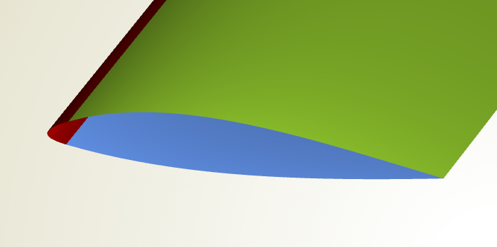
If you now create a 3D surface (say a lofted surface or a meta surface) from such a profile, you can directly split the gen­er­ated surface in order to have the indi­vid­ual surface patches avail­able. This is helpful when you need to split a single 3D surface into several pieces e.g. for more control in the meshing process and the sim­u­la­tion. See the fol­low­ing screenshot:

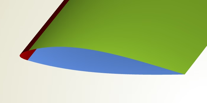
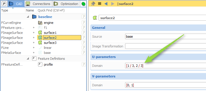
In this example, three image surfaces are created based on the single 3D surface. The next screen­shot shows how the second surface i.e. the leading edge gets defined:

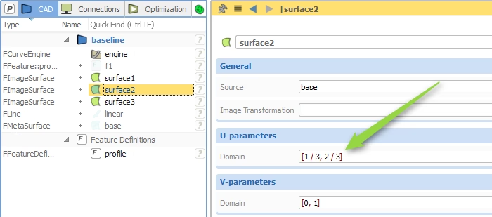
The surface u‑direction (“U‑parameters”) cor­re­sponds to the profile def­i­n­i­tion, while the v‑direction is the sweep direc­tion in this demo example. Just for inter­ested readers and to complete this short blog post: Check out the feature def­i­n­i­tion of the profile from which the single surface gets created…

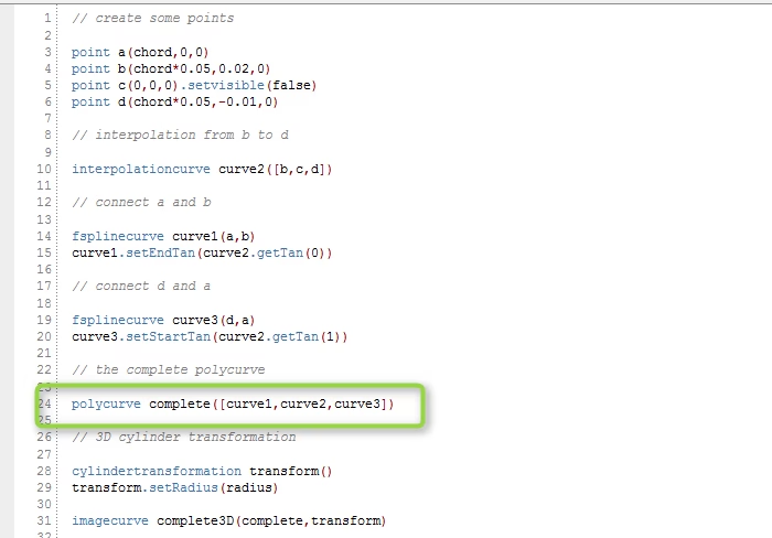
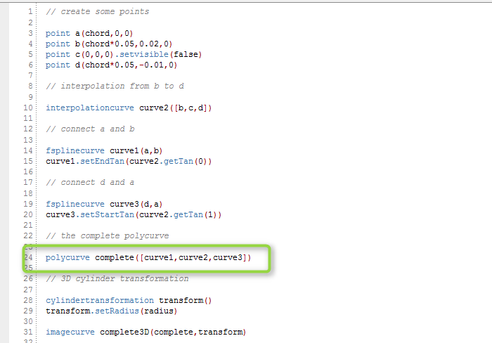
The poly­curve receives the 3 input curves (fsplinecurve, inter­po­la­tion­curve, fsplinecurve) which is high­lighted in the final screen­shot. The profile is then trans­formed into the 3D space by using a cylinder trans­for­ma­tion. Don’t get scared by the feature pro­gram­ming language — you can set up such a simple example also in the graph­i­cal user inter­face of CAESES®, inter­ac­tively and without any further pro­gram­ming know-how :-)

More Infor­ma­tion

Do you like this short article? Then please share it with your friends or col­leagues. Also check out our product pages for more infor­ma­tion about CAESES®.