How To Create a Response Surface in 4 Easy Steps
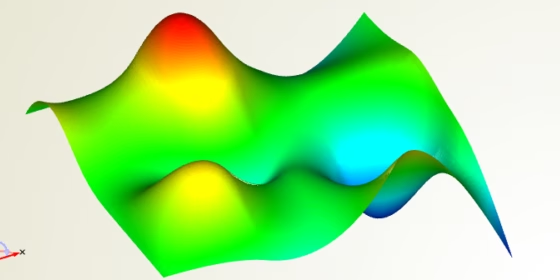
Response surfaces, also known as surrogate models or meta models, are nowadays often used whenever the evaluation of a function is not directly possible or simply too expensive. In the context of engineering and simulation, a typical application is the use of response surfaces instead of expensive CFD computations. The simulation of new design candidates, such as a new ship hull shape or a new aircraft wing design, can take hours or even days to complete. Naturally, fully automated and comprehensive design optimization is then out of reach.
Simulations can take hours or even days to complete. How can we efficiently find an optimal design?
To overcome this barrier, the idea is to simulate only a sufficiently small number of samples and create a response surface based on this pre-computed or experimental data. With such a response surface, one can efficiently run further studies or optimizations with thousands of function calls without triggering the expensive simulation code again. Famous mathematical approaches for response surfaces are polynomial models, kriging (Gaussian process), radial basis functions and neural networks. So how can we now create and employ such a response surface in CAESES®, based on an existing data set with samples for variable and function values?
Step #1: Create a new project
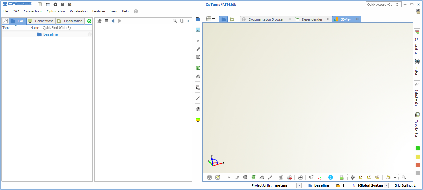
Open CAESES® and save a new project somewhere to your PC. Everyone can probably handle this step ;-)
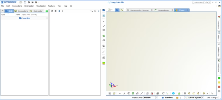
Save a new CAESES project
Step #2: Provide the data base
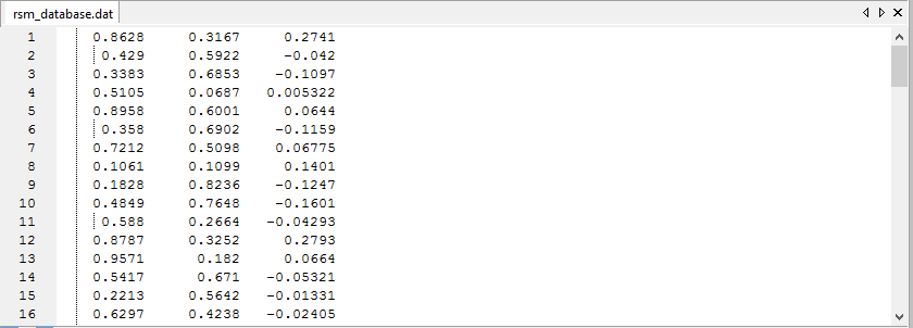
Now we need a data base with samples that gives us the variable values along with the corresponding function values i.e existing evaluations. For instance, this could be shape parameters along with some CFD or other simulation results. We keep the format simple: just provide an ASCII file with N rows where the variable values are listed, followed by the evaluations. Here is an example with N=16 samples, 2 variables and 1 objective function (which is given in the last column):
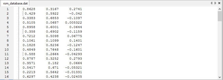
Provide a simple data base as ASCII file - each row represents 1 sample data
Put this file into the current project directory, i.e. where you stored your project file. That’s all for the data base.
Step #3: Create the response surface
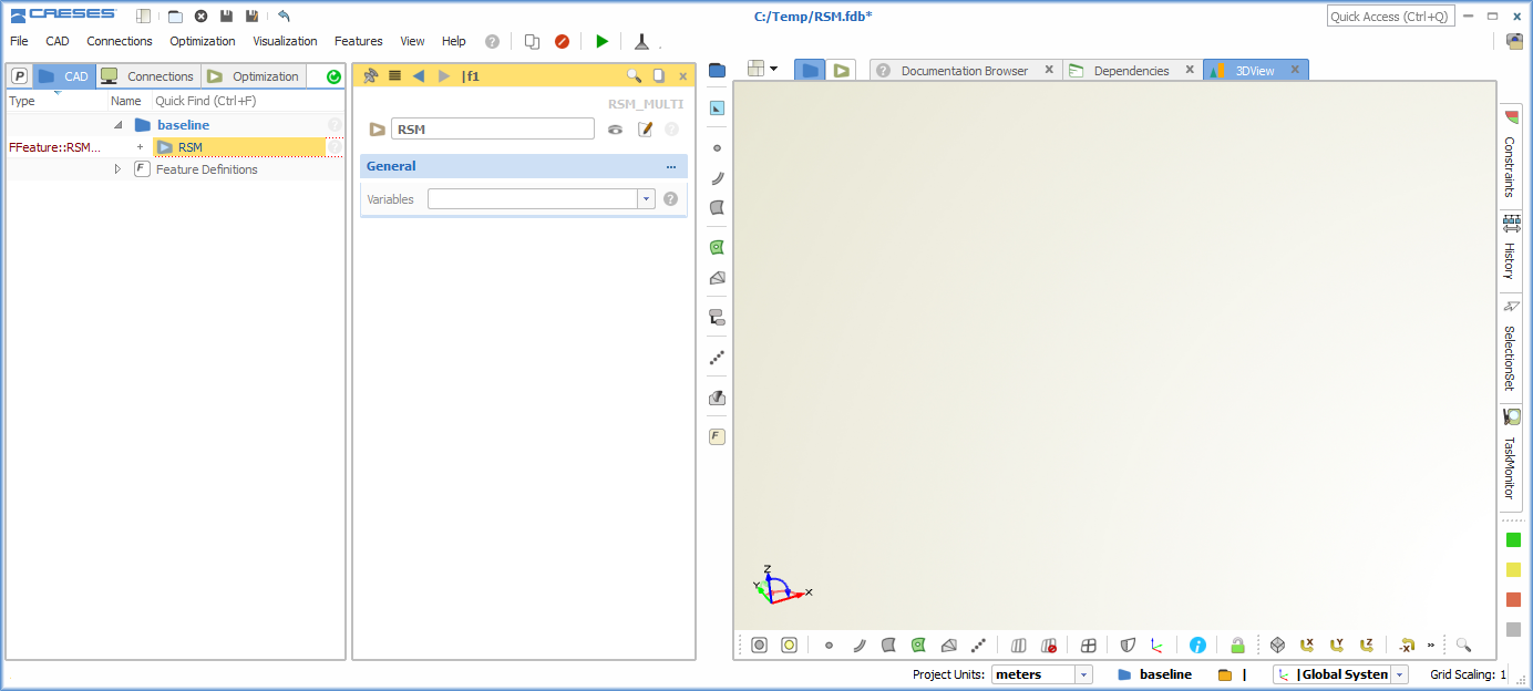
Use our response surface feature and drag & drop it into the graphical user interface so that it appears in the object tree of CAESES®.
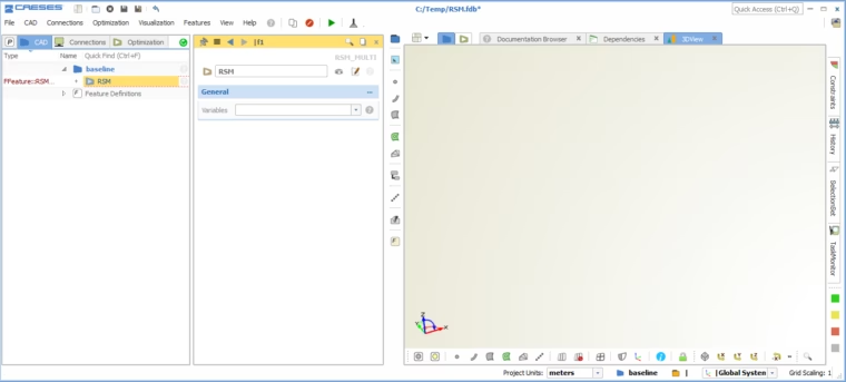
Create response surface object in the tree
Step #4: Perform a calculation on the response surface
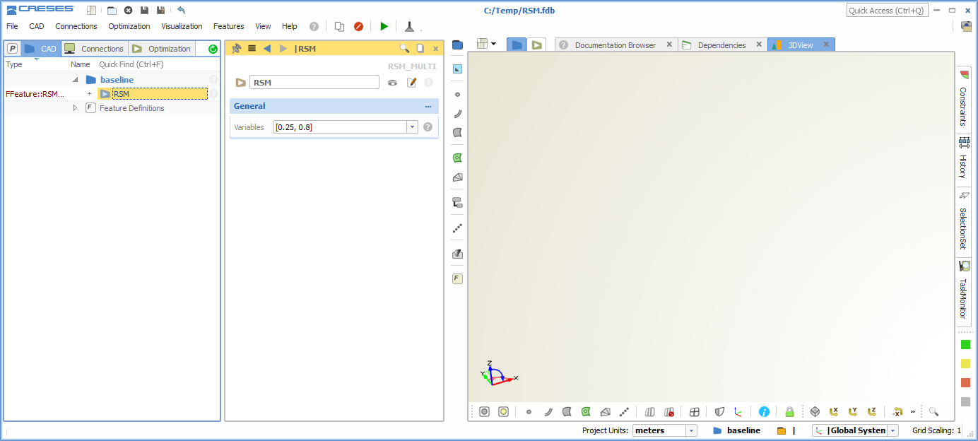
In the next step, enter your variable values into the editor for which you want to receive the calculated function value. Note that we use the list syntax with the brackets ([element1, element2,…]). In our example, we enter two values for the two variables, respectively.
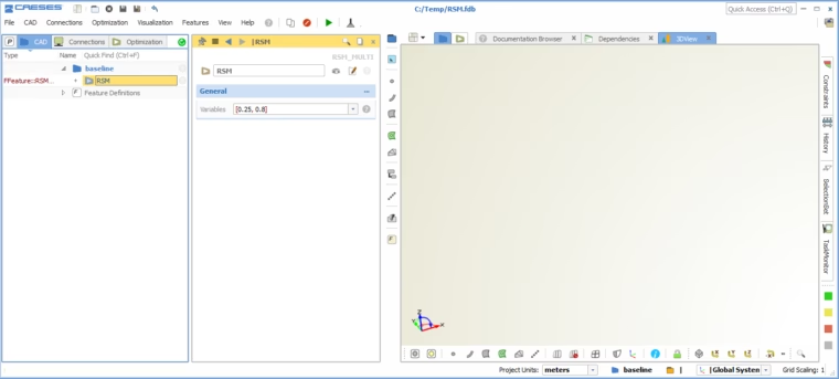
Enter variable values to perform a calculation on the response surface
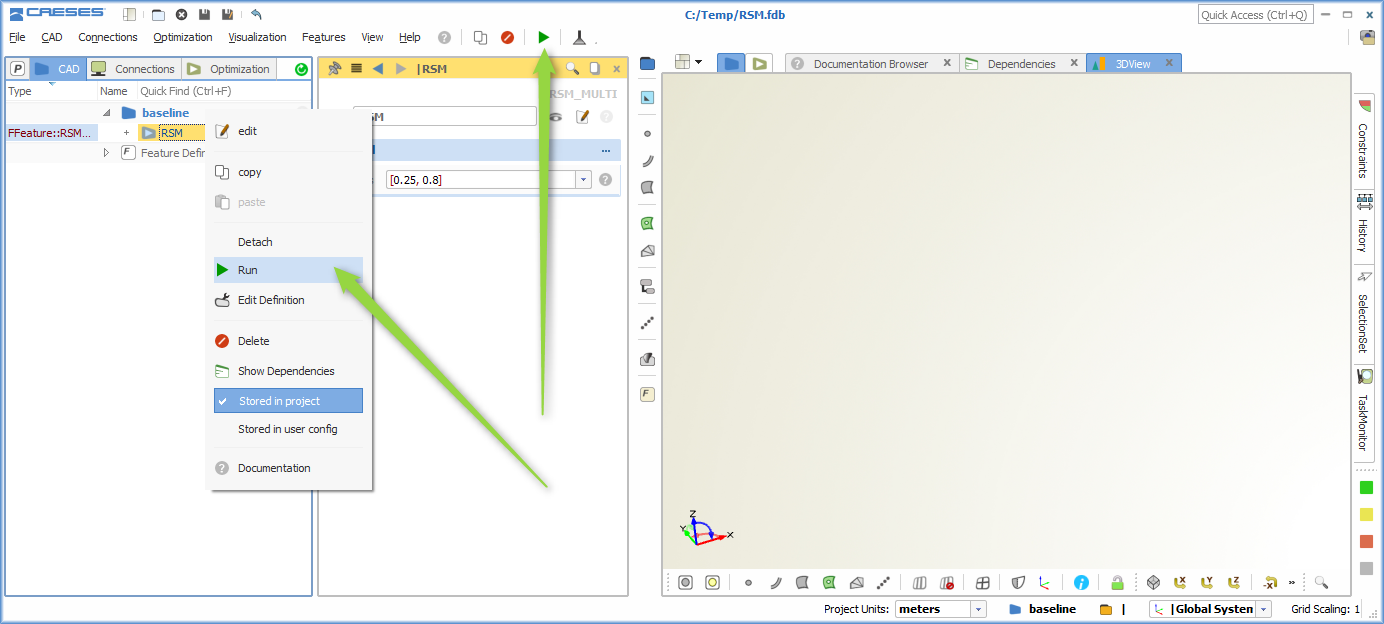
Trigger the creation of the model and the function evaluation either through the context menu, or through the green “play” button at the top of the window (there won’t be music starting up by pressing this button, just FYI …).
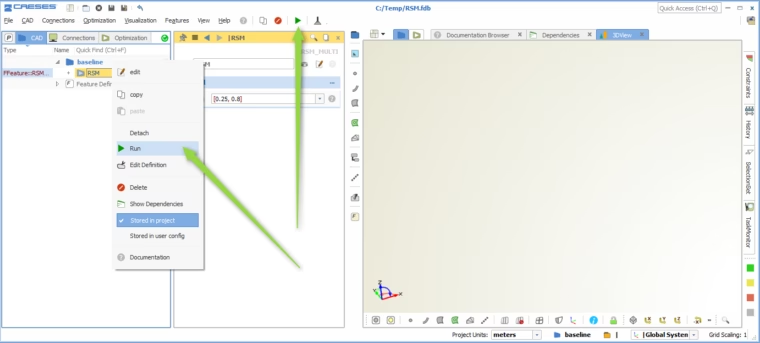
Perform the evaluation on the response surface
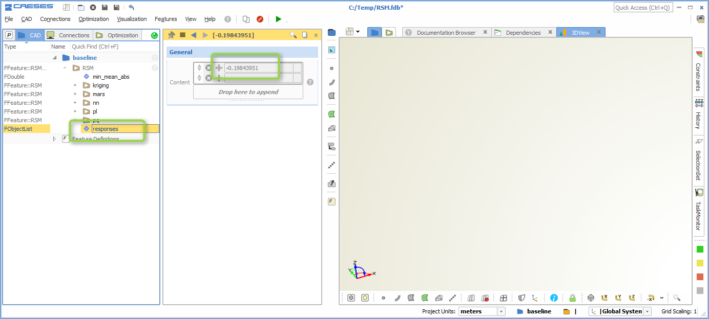
That’s it. The result is now immediately given in the tree when you expand the “RSM”-node:
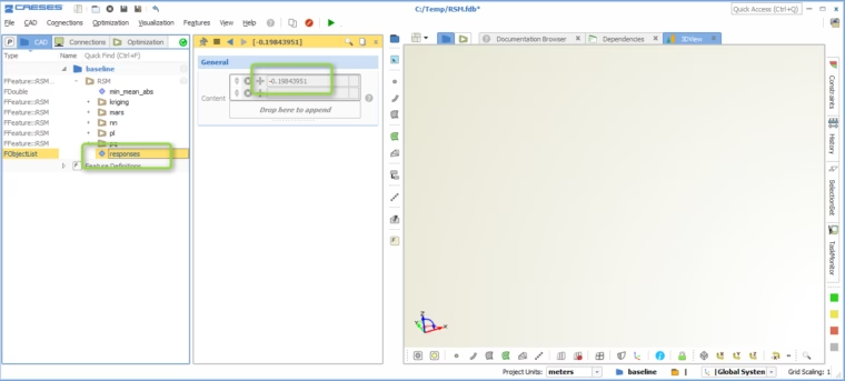
The evaluations are finally given as a list, which in our basic example is a single value
For this blog post, we used some sort of multi-model approach where several different response surface models are checked automatically. The one with the best fit is finally taken for performing the evaluation. By generating a set of different metrics such as absolute errors, mean values, R2 etc., you can optionally control how to pick the model.
What’s Next?
At this stage, you have a very basic editor to enter your variable values (and it’s a bit boring and tedious to manually enter the values). Hence, as a next step, you would create design variable objects and parameters for your evaluation, see the screenshot below. This allows you to run further automated studies or formal optimizations with CAESES® on the response surface. For fully automated surrogate-based optimiziation in CAESES® with design engines, you can also check out the post “Global Optimization using Response Surfaces”
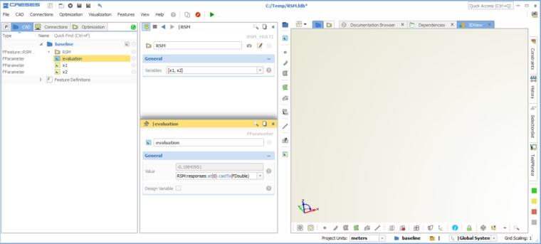
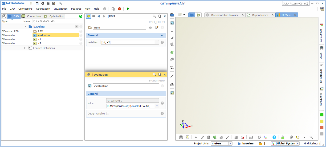
Introduce parameters and design variables, e.g. for automated studies