Optimization of a Leading Edge for Flat Plate Boundary Layer Experiments
This blog post is part of our CAESES Student Award 2020 competition about the use of CAESES in academia, where we showcase exciting material submitted to us by students who use CAESES in their research. Many students from high school to PhD make use of CAESES to reach their project goals. If you are one of them, we encourage you to send us an article about your project and how CAESES has helped you. Interesting articles will be posted regularly in our blog, along with some information about the author, and at the end of February 2021, we will select the best author, who will win some exciting prizes.
Predicting the transitional boundary layer is still an almost impossible task for arbitrary flow conditions. The consideration of the impact of boundary conditions such as pressure gradient, free-stream turbulence and surface roughness demand improved transition models, which are the interest of a research group at the Karlsruhe University for Applied Sciences.
The Importance of the Leading Edge
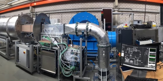
In order to investigate the transition from laminar to turbulent boundary layer flow, the researchers have built their own wind tunnel, including a flat plate test section and exchangeable contoured top and bottom walls. The latter offer the possibility to generate either generic or realistic (e.g. gas turbine blade) pressure distributions along the flat plate. In the closed-loop wind tunnel, the air coming from the compressor flows into the settling chamber, where honeycombs and sieves eliminate large turbulent eddies and homogenize the flow. A further homogenization is reached by the nozzle that accelerates the flow and guides it into the turbulence generator, which consists of horizontal and vertical baffle plates. By rotating those plates and adjusting the streamwise position of the grid, the desired turbulence intensity and turbulent length scale of the flow can be set independently of each other. This offers the possibility to investigate a wide range of flow conditions. The flow then enters the measuring section, from where it flows through an air cooler and back to the compressor.
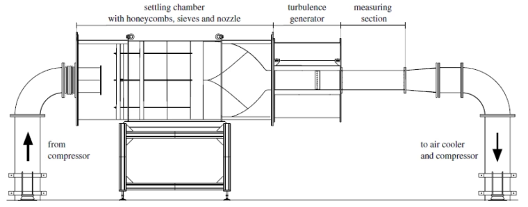
Schematic of the wind tunnel at the Karlsruhe University of Applied Sciences by Gramespacher et al. (2019), "The generation of grid turbulence with continuously adjustable intensity and length scales”, Experiments in Fluids (2019) 60:85, Springer-Verlag GmbH Germany.
For a long time, the standard in experimental boundary layer investigations was to use either sharp or elliptically shaped leading edges. It was assumed that the effect of the leading edge on the experimental results measured downstream is negligible. In recent years, however, several research groups have shown that the leading edge has a more significant impact on boundary layer stability than previously thought. Especially adverse pressure gradients destabilize the laminar boundary layer due to an amplification of naturally occurring disturbances. Therefore, the onset of laminar-turbulent transition moves upstream. The disadvantage of elliptical leading edges is twofold. Firstly, close downstream of the edge nose, the pressure gradient is adverse, and secondly, the junction between the leading edge and the flat plate presents a discontinuity in curvature. Both features contaminate the experimental results downstream of the leading edge. In previous experiments by the research group, the leading edge influence could be minimized by using a nozzle that induces a favorable pressure gradient along the leading edge and the subsequent flat plate. The focus of further research projects, however, is on unaccelerated free-stream flows. This demands an optimized leading edge, where the optimum is characterized as a pressure gradient that is zero as far upstream as possible and nowhere adverse. In order to evaluate the flow behavior of a leading edge, the dimensionless pressure coefficient 𝐶𝑝 is introduced as
Optimizing the Contour
CAESES was introduced to optimize the leading edge contour. It is designed as a B‑Spline with 11 control points, while the resulting geometry is exported as an STL-file. The multidimensional optimization starts with a global search for an optimal leading edge using the MOSA (Multi-Objective Simulated Annealing) algorithm, followed by a local search with TSearch algorithm. The length of the leading edge 𝑎 is defined as the distance from the leading edge nose to the junction with the flat plate. The thickness 𝑑 is the flat plate thickness.
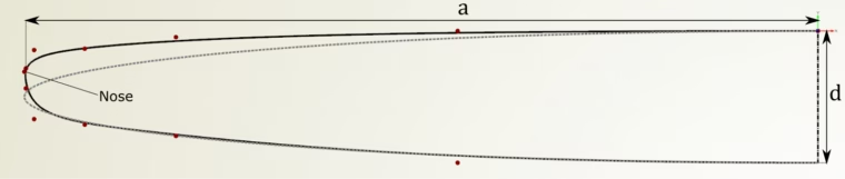
Leading edge contour realized with a B-Spline with 11 control points (solid line). The plate length 𝑎 and thickness 𝑑 are illustrated. The contour of a symmetric 12:1 ellipse is shown as a dotted line (see Results for further info on the ellipse).
Geometric Constraints
The researchers intend to run hot film sensor measurements along the flat plate surface at arbitrary streamwise positions. The hot film sensor is mounted on a movable steel belt (30 μm thick), which surrounds the flat plate including the leading edge. A stepper motor drags the steel belt around the plate to adjust the streamwise position of the hot film sensor. To ensure an undisturbed flow over the leading edge, the belt needs to fit tightly around the leading edge contour. Unfortunately, a sharp leading edge would deform the belt permanently. Consequently, the maximal curvature of the leading edge was limited by a geometric constraint. A maximal curvature is converted to a minimal radius of curvature, whose corresponding circle is illustrated in the following figure. Preliminary experiments have shown that a minimum radius of curvature of approximately 2.5 mm should prevent plastic deformation of the steel belt.
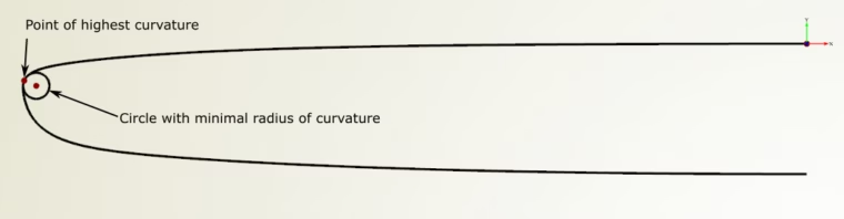
The circle corresponding to the minimal radius of curvature is found where the curvature of the leading edge has its maximum.
CFD Coupling with OpenFOAM
The researchers coupled CAESES with the open source CFD library OpenFOAM. To ensure parallel stream lines along the flat plate, the stagnation point has to be at the leading edge nose. By increasing the outlet pressure above the plate, while the outlet pressure below the plate remains unaffected, the position of the stagnation point can be adjusted towards the top of the leading edge. It can be moved downwards by decreasing the upper outlet pressure. An optimization process ensures the position of the stagnation point to be at the leading edge nose. The resulting pressure contours as well as the stagnation point are shown below.
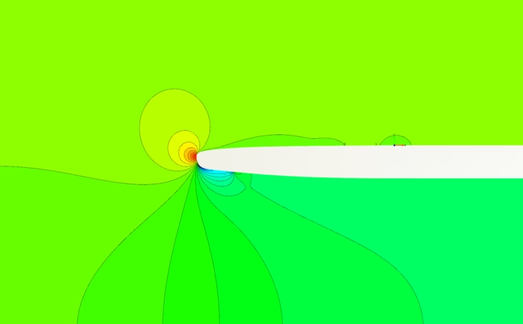
Pressure contours around the optimized flat plate leading edge. The stagnation point is positioned correctly at the nose of the leading edge.
Results
In order to clarify the improvements achieved by the optimization method, the optimized leading edge contour is compared with two ellipses. The first one is a 12:1 ellipse, which means its semi-major axis is 12 times longer than the semi-minor axis. It has the same length 𝑎 as the optimized plate contour. It does not fulfill the geometric constraint described above, since the minimal radius of curvature is too small (≈ 1.0 mm). The second ellipse is a 5:1 ellipse and is significantly shorter, but fulfills the geometric constraint with a minimal radius of curvature of 2.5 mm.
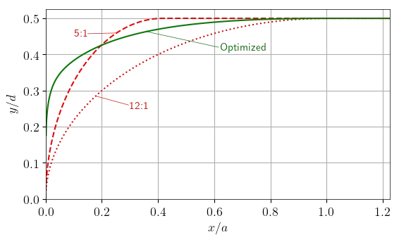
Contour of the optimized leading edge compared with the 5:1 and the 12:1 ellipses. The 𝑦 and 𝑥 values were normalized by height of the plate d and the leading edge length 𝑎, respectively.
The following figure shows the dimensionless pressure distribution for all three edge contours. For the optimized leading edge, the pressure gradient is zero and constant at about 40% of the edge length 𝑎. The small adverse pressure gradient downstream of the nose is negligible compared to that of the ellipses, as it occurs only close to the nose. Contrarily, for both ellipses, the pressure gradient is non-zero well downstream of the edge nose, indicated by a rising pressure coefficient 𝐶𝑝. For the 5:1 ellipse, 𝐶𝑝 has a minimum at approximately 𝑥/𝑎 = 0.2, resulting in an adverse pressure gradient between 𝑥/𝑎 = 0.2 and 𝑥/𝑎 = 1.0. Although the 12:1 ellipse induces a much smoother 𝐶𝑝 distribution, it still has a minimum even further downstream at approximately 𝑥/𝑎 = 0.8. This results in an adverse pressure gradient until the end of the simulation domain at 𝑥/𝑎 = 1.2 that may reach far into the measurement section. Although the adverse pressure gradient is quite small, this would result in decelerated free-stream flow, affecting the experimental results.
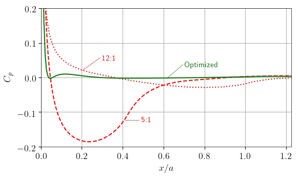
Pressure coefficient 𝐶𝑝 over the downstream position x normalized by the leading edge length 𝑎.
The optimization process is shown in the following animation, where both the variation of the contour and the resulting pressure coefficient distribution are displayed. It shows clearly that even small variations in the contour can highly affect the resulting pressure coefficient. This requires a high manufacturing accuracy during the production of the optimized leading edges.
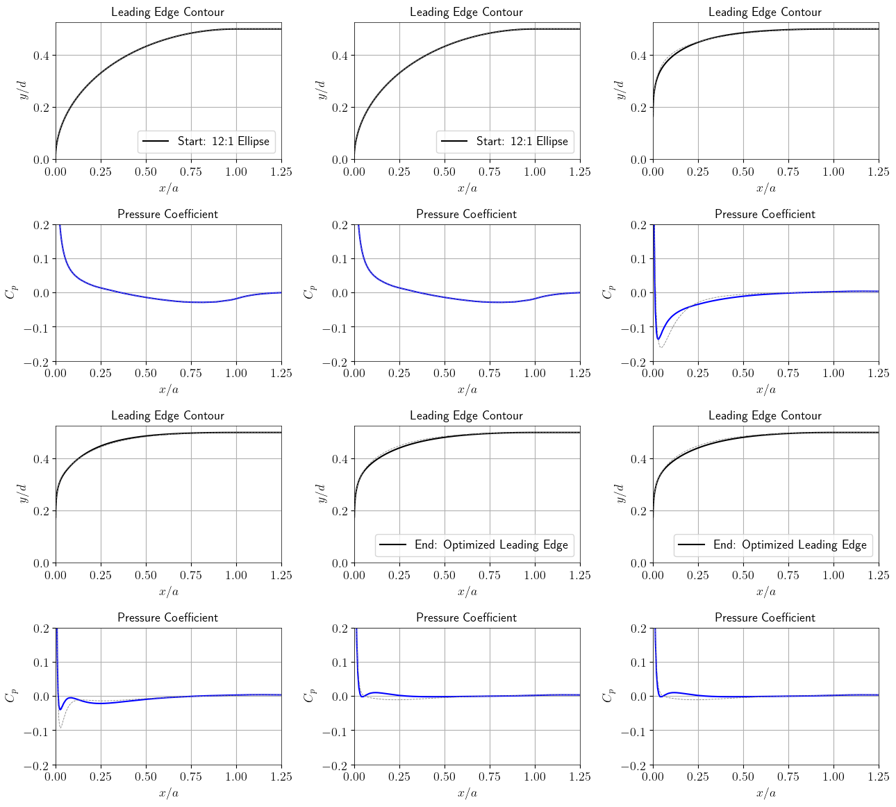


Optimization process of the leading edge contour. The starting design is the 12:1 ellipse. Then six different designs are shown, subsequently improving the quality function 𝐶𝑝. The final frame shows the optimal leading edge design.
Conclusion
CAESES helped optimizing the contour of the leading edge of a flat plate by varying the control points of the B‑Spline contour. The distribution of the pressure coefficient 𝐶𝑝 served as an objective function, such that it reached a constant value of zero as far upstream as possible. The pressure gradient is only slightly adverse directly downstream of the optimized leading edge nose. The geometric constraint of a minimal radius of curvature probably prevents a leading edge with a more ideal pressure gradient distribution. Compared to the two ellipses, the new design of the leading edge is clearly superior.
About the Author
Thanks a lot to Philipp Masino and his colleagues from Karlsruhe University of Applied Sciences, for submitting this interesting article and images about their research and optimization with CAESES.

Philipp Masino graduated from the Karlsruhe Institute of Technology in Industrial Mathematics and is now working as PhD student at the Karlsruhe University of Applied Sciences. His research field is the impact of high pressure gradients, high free-stream turbulence as well as surface roughness on transitional boundary layer flow. He is developing new computational models that can predict the onset and length of transition with respect to the impact of the above-mentioned parameters. These models are based on experimental data like heat transfer distributions, turbulent spot kinematics or detailed free-stream turbulence data measured in the research group’s wind tunnel. Furthermore, the group performs direct numerical simulations to support the experimental data.
Philipp Masino
PhD student at the Karlsruhe University of Applied Sciences